This is Part 1 - Reproducibility in Machine Learning - Research and Industry of technical blog series titled [Reproducibility in Machine Learning]. Part 2 & Part 3 can be found here & here respectively.
Machine learning (ML) is an interesting field aimed at solving problems that can not be solved by applying deterministic logic. In fact, ML solves problems in logits [0, 1] with probabilities! ML is a highly iterative and fiddly field with much of its intelligence derived from data upon application of complex mathematics. Sometimes, even a slight change such as changing the order of input/data can change the outcome of ML processes drastically. Actually xkcd quite aptly puts it:
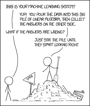 Figure 1: Machine Learning explained by XKCD
This phenomenon is explained as Change Anything Changes Everything a.k.a. CAKE principle coined by Scully et. al in their NIPS 2015 paper titled ["Hidden Technical Debt in Machine Learning Systems"][scully_2015]. CAKE principle highlights that in ML - no input is ever really independent.
Reproducibility as per the Oxford dictionary is defined as something that can be produced again in the same way. 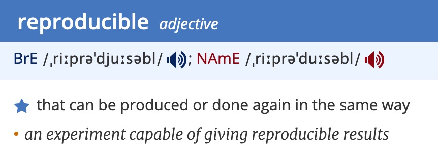 Figure 2: Reproducible defined
In ML context, it relates to getting the same output on the same algorithm, (hyper)parameters, and data on every run.
To demonstrate, let's take a simple linear regression example (shown below) on Scikit Diabetes Dataset. Linear regression is all about fitting a line i.e. Y = a + bX over data-points represented as X, with b being the slope and a being the intercept.
import matplotlib.pyplot as plt
import numpy as np
from sklearn import datasets, linear_model
from sklearn.metrics import mean_squared_error, r2_score
from sklearn.model_selection import train_test_split

diabetes = datasets.load_diabetes()
diabetes_X = diabetes.data[:, np.newaxis, 9]
xtrain, xtest, ytrain, ytest = train_test_split(diabetes_X, diabetes.target, test_size=0.33)
regr = linear_model.LinearRegression()
regr.fit(xtrain, ytrain)
diabetes_y_pred = regr.predict(xtest)

# The coefficients
print(f'Coefficients: {regr.coef_[0]}\n'
      f'Mean squared error: {mean_squared_error(ytest, diabetes_y_pred):.2f}\n'
      f'Variance score: {r2_score(ytest, diabetes_y_pred):.2f}')
# Plot outputs
plt.scatter(xtest, ytest,  color='green')
plt.plot(xtest, diabetes_y_pred, color='red', linewidth=3)
plt.ylabel('Quantitative measure of diabetes progression')
plt.xlabel('One of six blood serum measurements of patients')
plt.show()
Above ML code is NOT reproducible. Every run will give different results: a) The data distribution will vary and b) Obtained slop and intercept will vary. See Figure 3.
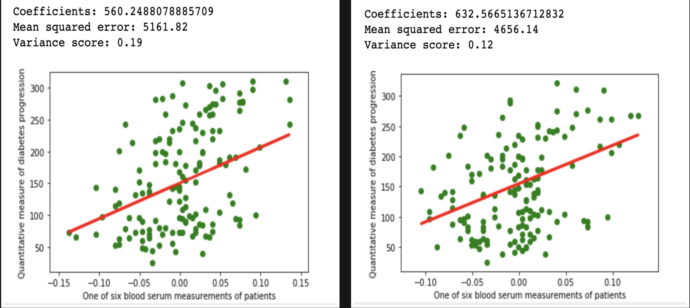 Figure 3: Repeated run of above linear regression code produces different results
In the above example, we are using the same dataset, same algorithm, same hyper-parameters. So why are we getting different results? Here the method train_test_split splits the diabetes dataset into training and test but while doing so, it performs a random shuffle of the dataset. The seed for this random shuffle is not set here. Because of this, every run produces different training dataset distribution. Due to this, the regression line slope and intercept ends up being different. In this simple example, if we were to set a random state for method train_test_split e.g. random_state=42 then we will have a reproducible regression example over the diabetes dataset. The reproducible version of the above regression example is as follows:
import matplotlib.pyplot as plt
import numpy as np
from sklearn import datasets, linear_model
from sklearn.metrics import mean_squared_error, r2_score
from sklearn.model_selection import train_test_split

diabetes = datasets.load_diabetes()
diabetes_X = diabetes.data[:, np.newaxis, 9]
xtrain, xtest, ytrain, ytest = train_test_split(diabetes_X, diabetes.target, test_size=0.33,
                                                random_state=42)
regr = linear_model.LinearRegression()
regr.fit(xtrain, ytrain)
diabetes_y_pred = regr.predict(xtest)

# The coefficients
print(f'Coefficients: {regr.coef_[0]}\n'
      f'Mean squared error: {mean_squared_error(ytest, diabetes_y_pred):.2f}\n'
      f'Variance score: {r2_score(ytest, diabetes_y_pred):.2f}')
# Plot outputs
plt.scatter(xtest, ytest,  color='green')
plt.plot(xtest, diabetes_y_pred, color='red', linewidth=3)
plt.ylabel('Quantitative measure of diabetes progression')
plt.xlabel('One of six blood serum measurements of patients')
plt.show()
Seeding random state is not the only challenge in writing reproducible ML. In fact, there are several reasons why reproducibility in ML is so hard to achieve. But I will go into that a bit later in section Challenges in realizing reproducible ML. The first question should be "why reproducibility matters in ML"?
Non-reproducible single occurrences are of no significance to science. - Popper (The Logic of Scientific Discovery)
The importance of reproducibility is increasingly getting recognized since Nature's Survey (2016) reported a reproducibility crisis. As per this survey report, 70% of researchers have failed to reproduce another scientist's experiments, and more than 50% have failed to reproduce their own experiments. With more than half of participating scientist agreeing to the presence of reproducibility crisis is indeed very real. Dr. Joelle Pineau, an Associate Professor at McGill University and lead for Facebook's Artificial Intelligence Research lab, covered the reproducibility crisis in her talk at International Conference on Learning Representations (ICLR) 2018 you tube. She is determined to nip
this crisis in bud from AI researchsrc. It's not just her, several AI research groups are coming up with measures to ensure reproducibility (example below): - Model Card at Google - Reproducibility Checklist at NeurIPS - ICLR Reproducibility Challenge at ICLR - Show your work at Allen Institute of Artificial Intelligence
Aside from being of no use if can't be reproduced, as Popper suggested in the above quote, why does reproducibility matter?
Reproducibility helps with understanding, explaining, and debugging. Reproducibility is also a crucial means to reverse engineering.
Machine learning is inherently difficult to explain, understand, and also debug. Obtaining different output on the subsequent run just makes this whole understanding, explaining, debugging thing all the more challenging. How do we ever reverse engineer? As it is, understanding and explaining are hard with machine learning. It's increasingly harder with deep learning. For over a decade, researches are have been trying to understand what these deep networks learn and yet have not 100% succeeded in doing so. 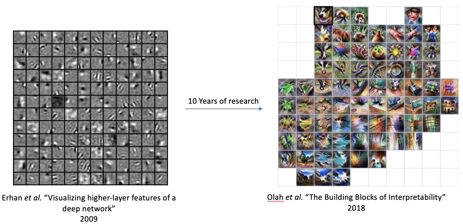
From visualizing higher layer features of deep networks year 2009 to activation-atlases i.e. what individual neurons in deep network do year 2017 to understanding how deep networks decides year 2018 - are all ongoing progressive efforts towards understanding. Meanwhile, explainability has morphed into a dedicated field 'Explainable Artificial Intelligence XAI.
If anything can go wrong, it will -Murphy's law
Correctness is important as Murphy's law rarely fails us. These are some of the examples of great AI failures of our times.
 Figure 4: Example of some of the great AI failures of our times
Google Photos launched AI capabilities with automatically tagging images. It was found to be tagging people of dark skin as gorillas. Amazon's recruiting software exhibiting gender bias or even IBM's Watson giving unsafe recommendations for cancer treatment.
ML output should be correct in addition to being explainable. Reproducibility helps to achieve correctness through understanding and debugging.
ML output must be credible. It's not just from a fairness, ethical viewpoint but also because they sometimes impact lives (e.g. mortgage approval). Also, end-users of ML output expect answers to verifiable, reliable, unbiased, and ethical. As Lecun said in his International Solid State Circuit Conference in San Francisco, 2019 keynote:
Good results are not enough, Making them easily reproducible also makes them credible. - Lecun, ISSCC 2019
Reproducibility in preceding layers is needed to build out and extend. Can we build a building outline model if we cant repeatedly generate roof semantics as shown in figure 5? What if we keep getting the different size for the same roof?  Figure 5: Extending ML
Extensibility is essential to utilizing ML outputs for consumption. As it is, raw outputs from ML are rarely usable by end-user. Most ML outputs need to be post-processed and augmented to be consumption ready.
The world's most valuable resource is no longer oil, but data! - economist.com
To train a successful ML algorithm large dataset is mostly needed - this is especially true for deep-learning. Obtaining large volumes of training data, however, is not always easy - it can be quite expensive. In some cases the occurrences of the scenario can be so rare that obtaining a large dataset will either take forever or is simply not possible. For eg. dataset for Merkel-cell carcinoma, a type of skin cancer that's very rare, will be very challenging to procure.
For this reason, data harvesting a.k.a. synthetic data generation is considered. Tirthajyoti Sarkar, the author of Data Wrangling with Python: Creating actionable data from raw sources, wrote an excellent post on data harvesting using scikit that covers this topic in detail. However, more recently, Generative Adversarial Networks (GAN) by Ian Goodfellow is being heavily used for this purpose. Synthetic Data for Deep Learning is an excellent review article that covers this topic in detail for deep-learning.
Give ML models e.g. (GAN) are being used to generate training data now, it's all the more important that reproducibility in such application is ensured. Let's say, we trained a near-perfect golden goose model on data (including some synthetic). But the storage caught proverbial fire, and we lost this golden goose model along with data. Now, we have to regenerate the synthetic data and obtain the same model but the synthetic data generation process is not quite reproducible. Thus, we lost the golden goose!
Reproducible ML does not come in easy. A wise man once said:
When you want something, all the universe conspires in helping you to achieve it. - The Alchemist by Paulo Coelho
But when it comes to reproducible ML it's quite the contrary. Every single resource and techniques (Hardware, Software, Algorithms, Process & Practice, Data) needed to realize ML poses some kind of challenge in meeting reproducibility (see figure 6).
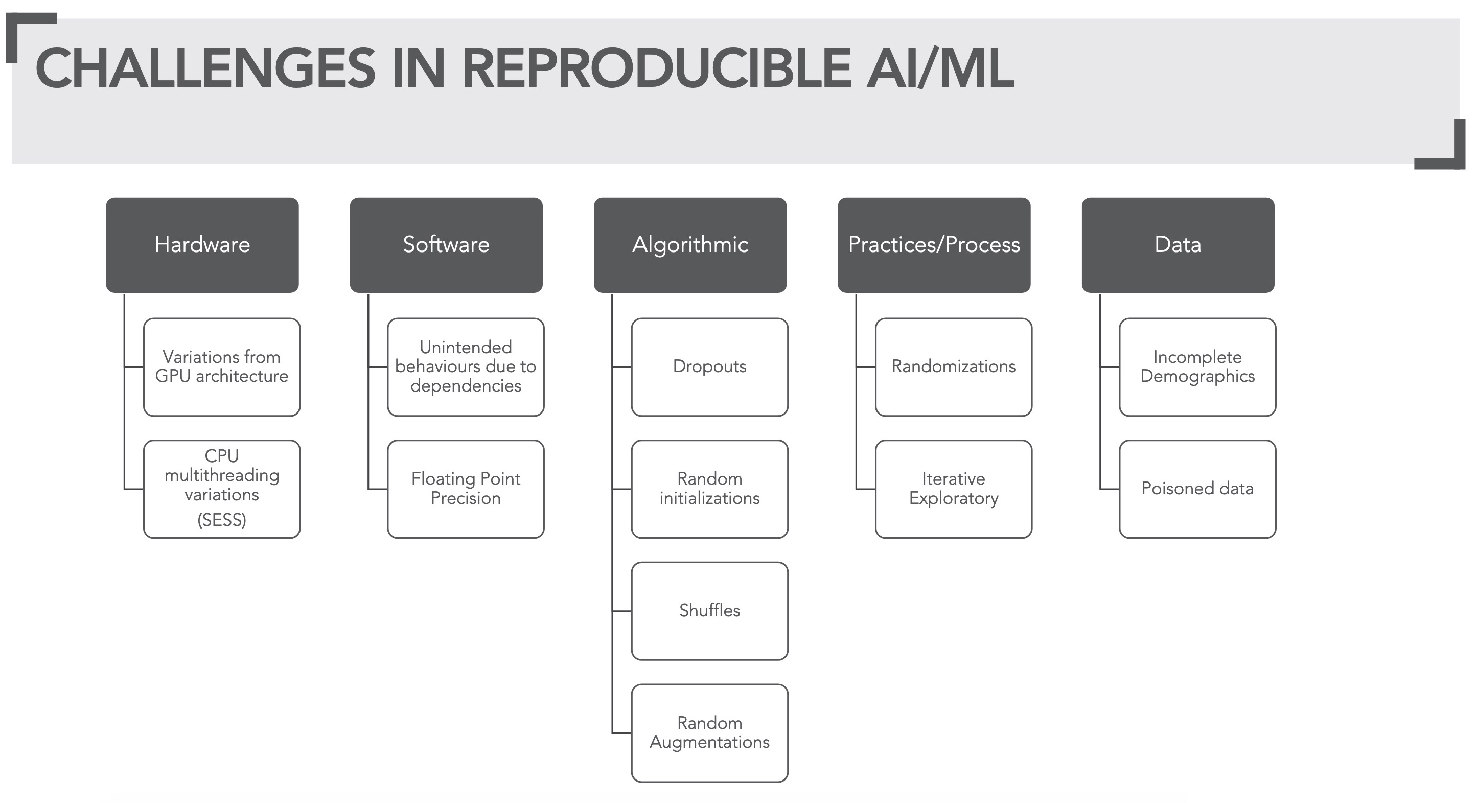 Figure 6: Overview of challenges in reproducible ML
ML algorithms are quite compute hungry. Complex computation needed by ML operation, now a day's runs in order of Giga/Tera floating-point operations (GFLOPS/TFLOPS). Thus needing high parallelism and multiple central processing Units (CPU) if not, specialized hardware such as (general purpose) graphics processing unit (GPU) or more specifically (GPGPU), tensor processing unit (TPU) etc. to complete in the reasonable time frame.
But these efficiencies in floating-point computations both at CPU & GPU level comes at a cost of reproducibility.
Using Intra-ops (within an operation) and inter-ops (amongst multiple operations) parallelism on CPU can sometimes give different results on each run. One such example is using OpenMP for (intra-ops) parallelization. See this excellent talk titled "Corden's Consistency of Floating Point Results or Why doesn't my application always give" Corden 2018 for more in-depth insight into this. Also see wandering precision blog.
General purpose GPUs can perform vector operations due to stream multiprocessing (SEM) unit. The asynchronous computation performed by this unit may result in different results on different runs. Floating multiple adders (FMAD) or even reductions in floating-point operands are such examples. Some algorithms e.g. vector normalization, due to reduction operations, can also be non-reproducible. See reproducible summation paper for more info.
Changing GPU architecture may lead to different results too. The differences in SEM, or architecture-specific optimizations are a couple of reasons why the differences may arise.
See Corden's Consistency of Floating-Point Results or Why doesn't my application always give the same answer for more details.
It's not just hardware. Some software's offering high-level abstraction or APIs for performing intensive computation do not guarantee reproducibility in their routines. For instance NVIDIA's popular cuda based deep learning library cudnn do not guarantee reproducibility in some of their routines e.g. cudnnConvolutionBackwardFilter>sup>ref. Popular deep learning libraries such as tensorflowref 1,ref 2, pytorchref also do not guarantee 100% reproducibility.
There is an excellent talk Duncan Riach, maintainer of tensorflow_determinism on Determinism in deep learning presented at GPU technology conference by NVIDIA 2019
Sometimes it's not just a trade-off for efficiency but simple software bugs that lead to non-reproducibility. One such example is this bug that I ran into resulting in different geo-location upon same computation when a certain library version was upgraded. This is a clear case of software bug but underlines the fact that reproducibility goes beyond just computation, and precision.
Several ML algorithms can be non-reproducible due to the expectation of randomness. Few examples of these algorithms are dropout layers, initialization. Some algorithms can be non-deterministic due to underlined computation complexity requiring non-reproducible measures similar to ones discussed in the software section. Some example of these are e.g. vector normalization, backward pass.
ML loves randomness!
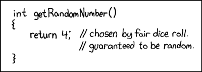 Figure 7: Randomness defined by xkcd
When things don't work with ML - we randomize (pun intended). We have randomness everywhere - from algorithms to process and practices for instance: - Random initializations - Random augmentations
- Random noise introduction (adversarial robustness) - Data Shuffles
To to ensure that randomness is seeded and can be reproduced (much like earlier example of scikit linear regression), with python, a long list of seed setting ritual needs to be performed:
os.environ['PYTHONHASHSEED'] = str(seed)
random.seed(seed)
tensorflow.random.set_seed(seed)
numpy.random.seed(seed)
tensorflow.keras.layers.Dropout(x, seed=SEED)
tensorflow.image.random_flip_left_right(x, seed=seed)
tensorflow.random_normal_initializer(x, y, seed=seed)
# many such algorithmic layers as aabove
Can we ever win with this seed setting?
 Figure 8: Seed setting (image credit: google)
No input is ever really independent. [Scully et. al 2015][scully_2015]
Data is the main input to ML algorithms and these algorithms are just compute hungry but also data-hungry. So we are really talking about big data. When data volume is large, we are dealing with all sorts of challenges: - Data management - Data provenance
- Data poisoning - Under-represented data (inappropriate demographic) - Over-represented data (inappropriate demographic)
One of the reasons why ML is so iterative because we need to evolve the ML algorithm with data whilst also continuously evolving data (e.g. data massaging, feature engineering, data augmentations). That's why data provenance is important but it's also important to maintain a linage with data provenance to ML processes. In short, an end to end provenance is needed with ML processes.
A model is rarely deployed twice. [Talby, 2018][Talby]
One of the reason for why a model rarely gets deployed more than once [ref][Talby] is Concept drift. Our concept of things and stuff keeps evolving. Don't believe me? figure 9 shows how we envisaged car 18's to now. Our current evolving impression of the car is solar power self-driving cars!
 Figure 9: Our evolving concept of
 car
So, now we don't just have to manage reproducibility over one model but many! Because our model needs to continually keep learning in a more commonly known term in ML as Continual learning more info. An interesting review paper on this topic is here.
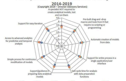 Figure 10: Top features - Dresner Advisory Services Data Science and Machine Learning Market Study
In fact, Continual learning is so recognized that support for easy iteration & continuous improvement were the top two features industry voted as their main focus with ML as per Dresner Advisory Services'6th annual 2019 Data Science and Machine Learning Market Study (see figure 10).
The next part of this technical blog series, [Reproducibility in Machine Learning], is Realizing reproducible Machine Learning - with Tensorflow.
[Reproducibility in Machine Learning]: /2019/12/20/Reproducibility-in-Machine Learning.html
[scully_2015]: https://papers.nips.cc/paper/5656-hidden-technical-debt-in-Machine Learning-systems.pdf
[Talby]: https://www.oreilly.com/radar/lessons-learned-turning-Machine Learning-models-into-real-products-and-services/
Figure 1: Version control explained by XKCD
Figure 2: Machine Learning end to end system
 Figure 3: Overview of challenges in reproducible ML
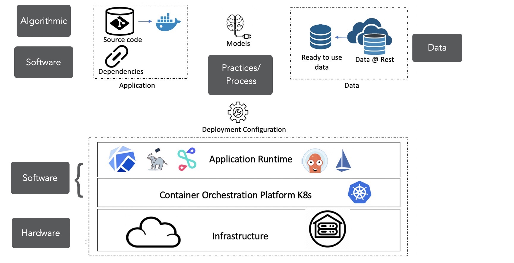 Figure 4: What to version control?
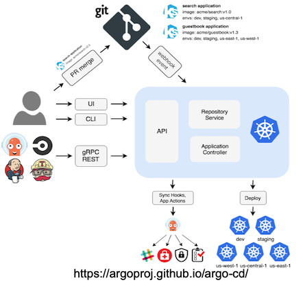 Figure 5: Gitops
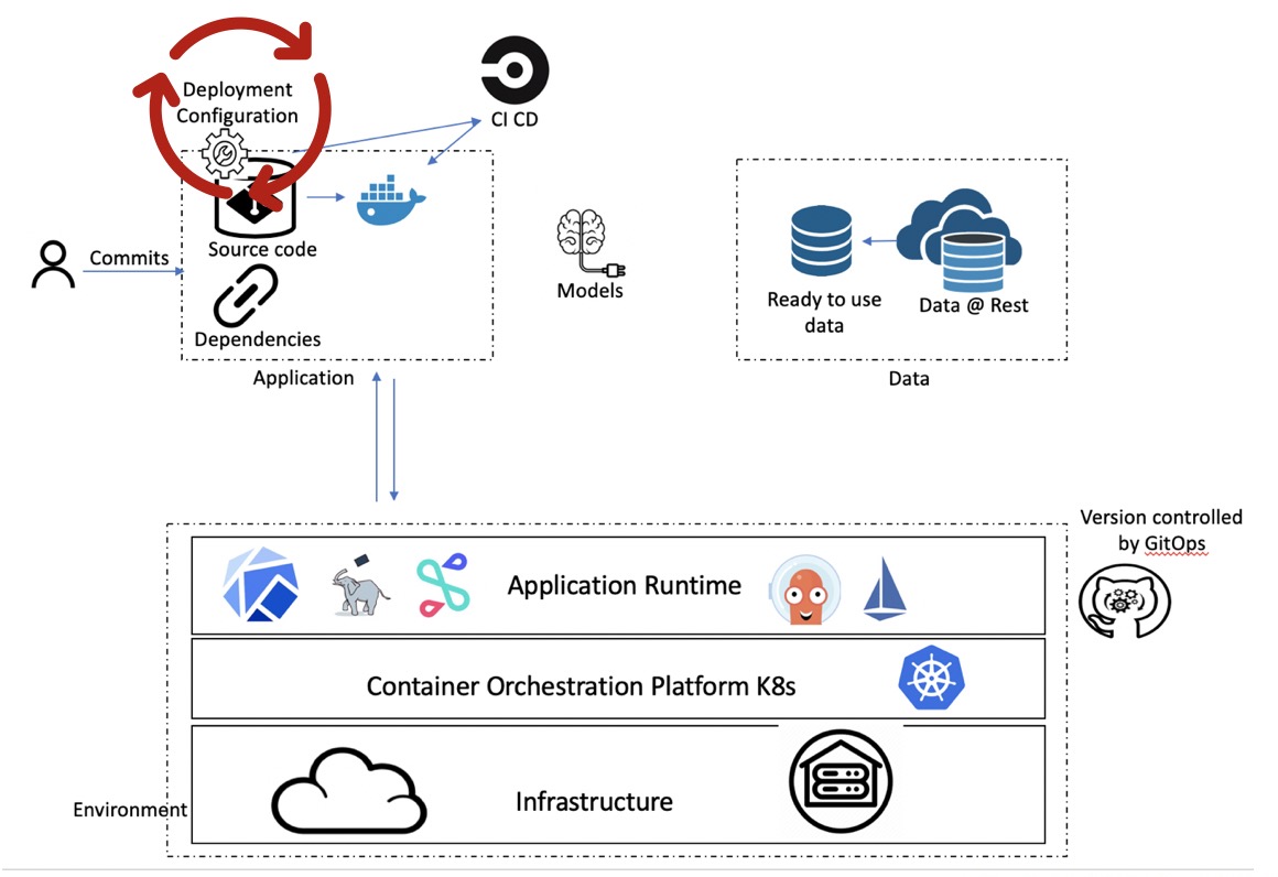 Figure 6: Gitops on environment config
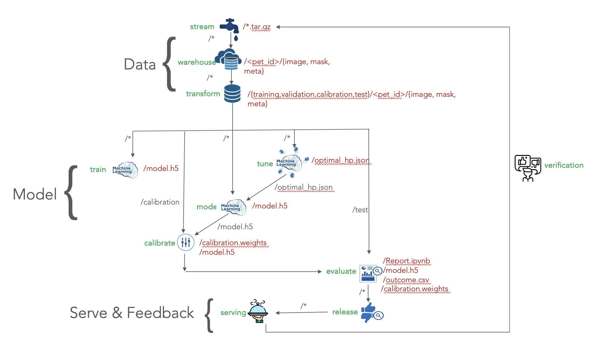 Figure 7: Artifact view of Machine Learning end to end system (shown in figure 2)
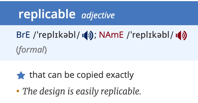 Figure 4: Replicability defined
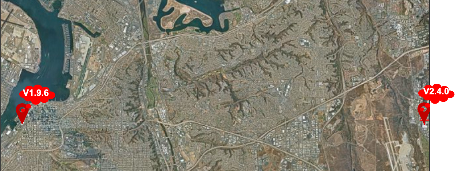 Figure 1: Example of why pinned libraries are important
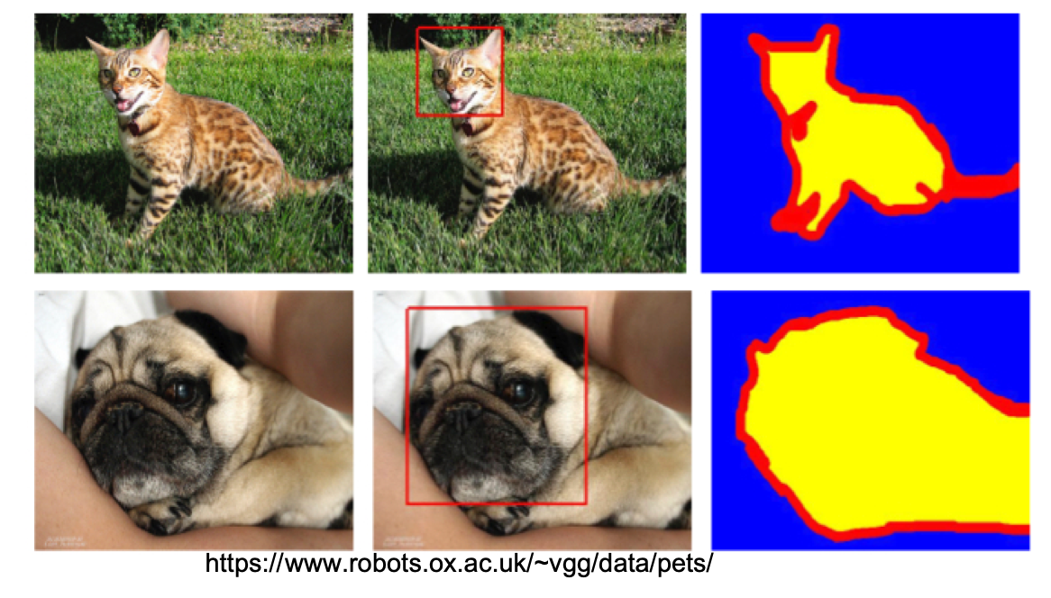 Figure 2: Oxford pet dataset
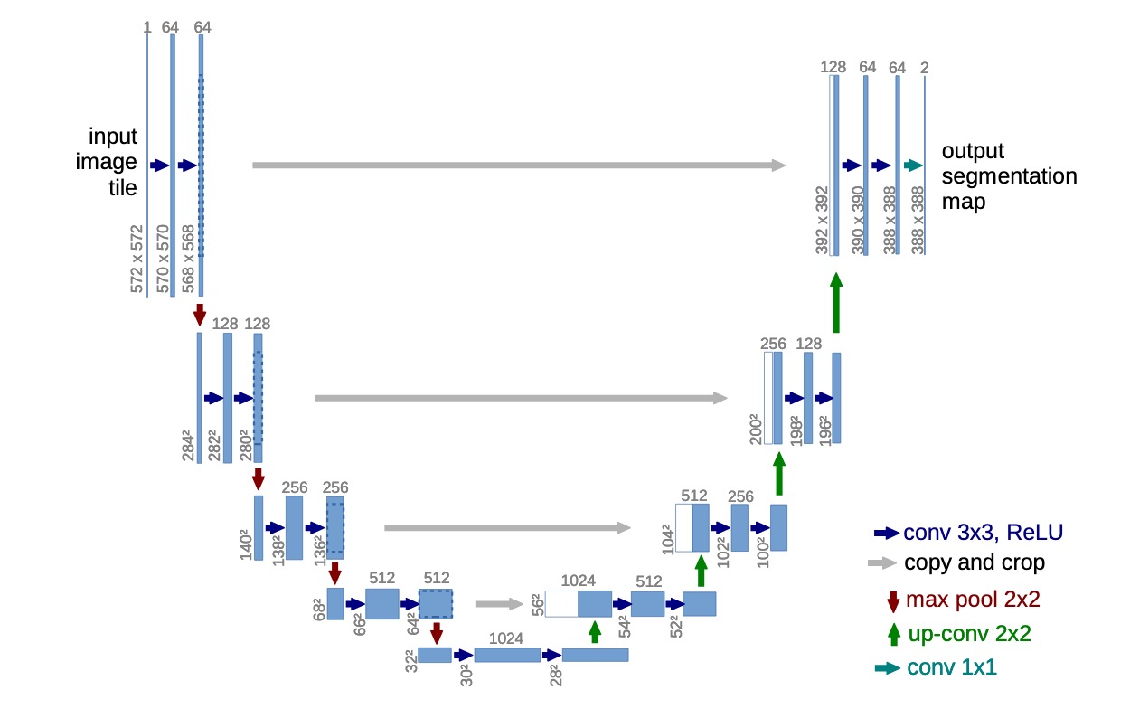 Fihure 3:
  Figure 4: Reproducible ML sample - semantic segmentation of oxford pet
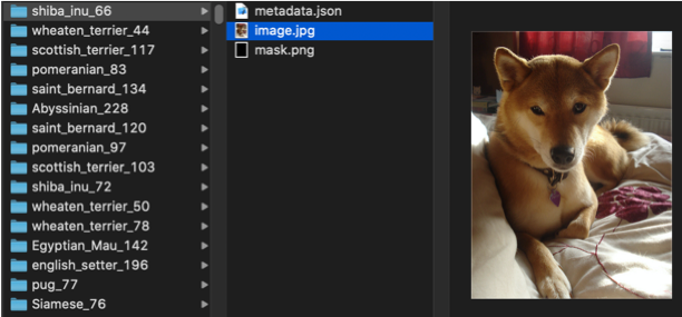 Figure 6: Pets data partitioned by Pets ID
 Figure 7: Pets data partitioned into training, validation, calibration, and test set
 Figure 8: NVIDIA release page snippet reproducibility
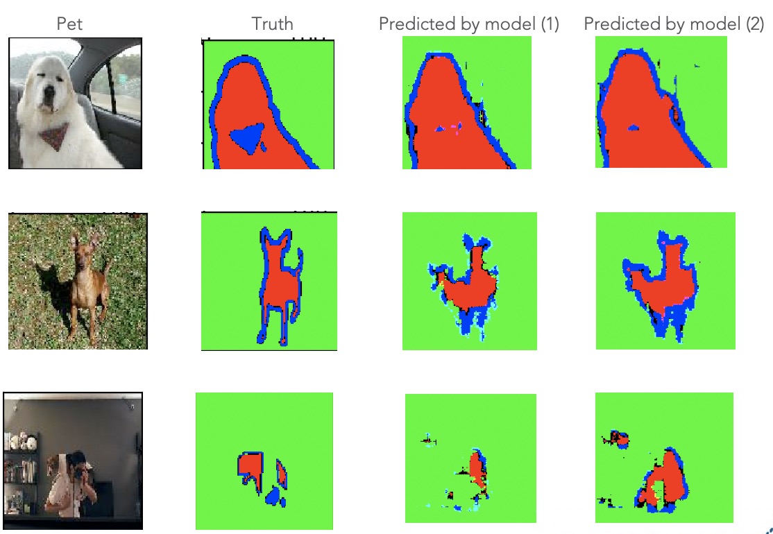 Figure 9: Effect of just forgetting to set one seed amidst many
 Figure 1: Machine Learning explained by XKCD
 Figure 2: Reproducible defined
 Figure 3: Repeated run of above linear regression code produces different results
 Figure 4: Example of some of the great AI failures of our times
 Figure 5: Extending ML
 Figure 7: Randomness defined by
  Figure 8: Seed setting (image credit: google)
 Figure 9: Our evolving concept of
  Figure 10: Top features - Dresner Advisory Services Data Science and Machine Learning