Skip to content

Data#

Review and comparison of two manifold learning algorithms: t-SNE and UMAP

What are manifold learning algorithms? What is t-SNE and UMAP? What are the differences between t-SNE and UMAP? How can I explore the features of a dataset using t-SNE and UMAP? These are my notes from my recent exploration into t-SNE and UMAP and trying to apply them to a multi-label dataset to understand the abilities and limits of these algorithms.

This post is broken down into the following sections:

Manifold learning algorithms (MLA)

For us humans, high-dimensional data are very difficult to visualize and reason with. That's why we use dimensionality reduction techniques to reduce data dimensions so that the data is easy to work with and reason about. Manifold learning algorithms (MLA) are dimensionality reduction techniques that are sensitive to non-linear structures in data. The non-linearity is what sets manifold learning apart from other popular linear dimensionality reduction techniques like Principal Component Analysis (PCA) or Independent Component Analysis (ICA). Non-linearity allows MLAs to retain complex and interesting properties of data that would otherwise be lost in linear reduction/projection. Because of this property, MLA is a very handy algorithm to analyze data - to reduce data dimensions to 2D or 3D, and visualize and explore them to find patterns in datasets.

t-SNE (t-Distributed Stochastic Neighbor Embedding) and Uniform Manifold Approximation and Projection UMAP are the two examples of MLA, that I will cover in this post. I will compare and contrast them and provide a good intuition of how they work and how to choose one over the other.

Note that, MLAs are tweaks and generalizations of existing linear dimensionality reduction frameworks themselves. Similar to linear dimensionality reduction techniques, MLAs are predominantly unsupervised even though supervised variants exist. The scope of this post is unsupervised techniques, however.

So what does non-linearity buys us? The following shows the difference in reduction using PCA vs t-SNE, as shown in McInnes excellent talk:

Comparison of t-SNE and UMAP on MNIST dataset. (Image from McInnes talk)

As we can see, PCA retains some structure. However, it is very well pronounced in t-SNE, and clusters are more clearly separated.

Neighbour graphs

t-SNE and UMAP are neighbor graph technique that models data points as nodes, with weighted edges representing the distance between the nodes. Through various optimizations and iterations, this graph and layout are tuned to best represent the data as the distance is derived from the "closeness" of the features of the data itself. This graph is then projected on reduced dimensional space a.k.a. embedded space. This is a very different technique than matrix factorization as employed by PCA, ICA for example.

t-Distributed Stochastic Neighbor Embedding (t-SNE)

t-SNE uses Gaussian joint probability measures to estimate the pairwise distances between the data points in the original dimension. Similarly, the student's t-distribution is used to estimate the pairwise distances between the data points in the embedded space (i.e. lower dimension or target dimension). t-SNE then uses the gradient descent technique to minimize the divergence between the two distributions in original and embedded space using the Kullback-Leibler (KL) divergence technique.

Perplexity in t-SNE is effectively the number of nearest neighbors considered in producing the conditional probability measure. A larger perplexity may obscure small structures in the dataset while small perplexity will result in very localized output ignoring global information. Perplexity must be less than the size of data (number of data points) then; otherwise, we are looking at getting a blobby mass. The recommended range for perplexity lies between 5-50, with a more general rule that the larger the data, the larger the perplexity.

Because of the use of KL divergence, t-SNE preserves the local structure in the original space, however, global structure preservation is not guaranteed. Having said that, when initialization with PCA is applied, the global structure is somewhat preserved.

Talking more about structures, the scale of distances between points in the embedded space is not uniform in t-SNE as t-SNE uses varying distance scales. That's why it is recommended to explore data under different configurations to tease out patterns in the dataset. Learning rate and number of iterations are two additional parameters that help with refining the descent to reveal structures in the dataset in the embedded space. As highlighted in this great distill article on t-SNE, more than one plot may be needed to understand the structures of the dataset.

Different patterns are revealed under different t-SNE configurations, as shown by distill article. (Image from distill).

t-SNE is known to be very slow with the order of complexity given by O(dN^2) where d is the number of output dimensions and N is the number of samples. Barnes-Hut variation of t-SNE improves the performance [O(dN log N)] however Barnes-Hut can only work with dense datasets and provide at most 3d embedding space. The efficiency gain in Barnes-Hut is coming from changes in gradient calculation which are done with O(n log n) complexity, that uses approximation techniques which leads to about 3% error in nearest neighbor calculation.

Because of these performance implications, a common recommendation is to use PCA to reduce the dimension before applying t-SNE. This should be considered very carefully especially if the point of using t-SNE was to explore into non-linearity of the dataset. Pre-processing with linear techniques like PCA will destroy non-linear structures if present.

Uniform Manifold Approximation and Projection UMAP

UMAP is based on pure combinatorial mathematics that is well covered in the paper and is also well explained by author McInnes in his talk and library documentation is pretty well written too. Similar to t-SNE, UMAP is also a topological neighbor graph modeling technique. There are several differences b/w t-SNE and UMAP with the main one being that UMAP retains not only local but global structure in the data.

There is a great post that goes into detail about how UMAP works. High level, UMAP uses combinatorial topological modeling with the help of simplices to capture the data and applies Riemannian metrics to enforce the uniformity in the distribution. Fuzzy logic is also applied to the graph to adjust the probability distance if the radius grows. Once the graphs are built then optimization techniques are applied to make the embedded space graph very similar to the original space one. UMAP uses binary cross-entropy as a cost function and stochastic gradient descent to iterate on the graph for embedded space. Both t-SNE and UMAP use the same framework to achieve manifold projections however implementation details vary. Oskolkov's post covers in great detail the nuances of both the techniques and is an excellent read.

UMAP is faster for several reasons, mainly, it uses random projection trees and nearest neighbor descent to find approximate neighbors quickly. As shown in the figure below, similar to t-SNE, UMAP also varies the distance density in the embedded space.

Manifold reprojection used by UMAP, as presented by McInnes in his talk. (Image from McInnes talk)

Here's an example of UMAP retaining both local and global structure in embedded space:

Example of UMAP reprojecting a point-cloud mammoth structure on 2-D space. (Image provided by the author, produced using tool 1)

Here's a side-by-side comparison of t-SNE and UMAP on reducing the dimensionality of a mammoth. As shown, UMAP retains the global structure but it's not that well retained by t-SNE.

Side by side comparison of t-SNE and UMAP projections of the mammoth data used in the previous figure. (Image provided by the author, produced using tool 1)

The explanation for this difference lies in the loss function. As shown in the following figure, UMAP uses binary cross-entropy that penalizes both local (clumps) and global (gaps) structures. In t-SNE however, due to KL Divergence as the choice of the cost function, the focus remains on getting the clumps i.e. local structure right.

Cots function used in UMAP as discussed in McInnes talk. (Image from McInnes talk)

The first part of the equation is the same in both t-SNE (coming from KL divergence) and UMAP. UMAP only has the second part that contributes to getting the gaps right i.e. getting the global structure right.

Comparison table: t-SNE vs UMAP

Characteristics t-SNE UMAP
Computational complexity O(dN^2)
(Barnes-Hut with O(dN log N) )
O(d*n^1.14)
(emprical-estimates O(dN log N))
Local structure preservation Y Y
Global structure preservation N
(somewhat when init=PCA)
Y
Cost Function KL Divergence Cross Entropy
Initialization Random
(PCA as alternate)
Graph Laplacian
Optimization algorithm Gradient Descent (GD) Stochastic Gradient Descent (SGD)
Distribution for modelling distance probabilities Student's t-distribution family of curves (1+a*y(2b))-1
Nearest neighbors hyperparameter 2^Shannon entropy nearest neighbor k

Exploring dataset with t-SNE & UMAP

Now that we have covered theoretical differences, let's apply these techniques to a few datasets and do a few side-by-side comparisons between t-SNE and UMAP.

Source code and other content used in this exercise are available in this git repository - feature_analysis. The notebook for MNIST analysis is available here. Likewise, the notebook for CIFAR analysis is available here.

Simple feature dataset like MNIST

The following figure reprojects MNIST image features on the 2D embedded space under different perplexity settings. As shown, increasing the perplexity, makes the local clusters very packed together. In this case, PCA based initialization technique was chosen because I want to retain the global structure as much as possible.

Reprojection of MNIST image features on the 2D embedded space using t-SNE under different perplexity settings. (Image provided by author)

It's quite interesting to see that the digits that are packed close together are: 1. 7,9,4 2. 3,5,8 3. 6 & 0 4. 1 & 2 5. That 6 is more close to 5 than 1 6. Likewise 7 is closer to 1 than 0.

At a high level this co-relation makes sense, the features of the digits that are quite similar are more closely packed than digitals that are very different. Its also, interesting to note that 8 and 9 have anomalies that map closely to 0 in rare cases in embedded space. So what's going on? Following image overlays randomly selected images on the clusters produced by t-SNE @ perplexity of 50.

Reprojection of MNIST image features on the 2D embedded space using t-SNE @ perplexity=50 with randomly selected image overlay. (Image provided by author)

As we pan around this image, we can see a distinct shift in the characteristics of the digits. For example, the 2 digits at the top are very cursive and have a round little circle at the joint of the two whereas as we travel to the lower part of the cluster of 2s, we can see how sharply written the bottom 2s are. The bottom 2s features are sharp angular joints. Likewise, the top part of the cluster of 1s is quite slanty whereas the bottom 1s are upright.

It's quite interesting to see that the 8's occasionally clustered together with 0's are quite round in the middle and do not have the sharp joint in the middle.

So, what does MNIST data look like with UMAP? UMAP's embedded space also reflects the same grouping as discussed above. In fact, UMAP and t-SNE clustering in terms of digits grouping are very much alike. It appears to me that UMAP and t-SNE are mirror reflections when it comes to how digits are grouped.

Reprojection of MNIST image features on the 2D embedded space using UMAP. (Image provided by author)

It's also very interesting to note how similar-looking 1s are that are reprojected to the same coordinates in the embedded space.

One example of samples that get reprojected to the same coordinates in the embedded space using UMAP. (Image provided by author)

Not all the data points that collide in embedded space will look exactly similar, the similarity is more in the reduced dimensional space. One such example is shown below. Here 1 and 0 are reprojected to the same coordinates. As we can see the strokes on the left side of 0 are very similar to strokes of 1. The circle of zero is not quite complete either.

One example of two different digits getting reprojected to the same coordinates in the embedded space using UMAP. (Image provided by author)

Here's also an example of samples falling into the same neighborhood in the embedded space that look quite distinct despite sharing some commonality (the strokes around the mouth of 4 and incomplete 8s)!

Example of 4 and 8s reprojected to the nearby coordinates in the embedded space using UMAP. (Image provided by author)

Its unpredictable what tangible features have been leveraged to calculate the similarities amongst data points in the embedded space. This is because the main focus of MLAs has been distance measures and the embedded space is derived based on best effort using unsupervised techniques with evident data loss (due to dimensionality reduction).

This was MNIST, where digits are captured with empty backgrounds. These are very easy cases because all the signals in the feature vectors are true signals that correspond to the digit as its drawn. When we start talking about visualizing data where there are noises in the signals then that case poses certain challenges. For example, taking the case of cifar dataset, the images of things are captured with a varying background as they are all-natural images unlike MNIST with a black background. In the following section, let's have a look at what happens when we apply t-SNE and UMA to the CIFAR dataset.

High-level differences between cifar and MNIST dataset. (Image provided by author)

More complex datasets like CIFAR

The following figure shows the resultant embedding of CIFAR images after applying UMAP. As shown below results are less than impressive to delineate amongst CIFAR classes or perform any sort of features analysis.

Results of CIFAR image feature visualization using t-SNE under different perplexity settings. (Image provided by author)

So, what's going on? Let's overlay the images and see if we can find some patterns and make sense of the one big lump we are seeing. The following figure overlays the image. It's really hard to find a consistent similarity between neighboring points. Often we see cars and vehicles nearby but not consistently. They are intermixed with flowers and other classes. It's simply too much noise in the feature vector to do any meaningful convergence.

Results of CIFAR image feature visualization using t-SNE. Shows images in an overlay on randomly selected points. (Image provided by author)

In the above two figures, we looked at analyzing CIFAR with t-SNE. The following plot is produced by using UMAP. As we can see it's not convincing either. Much like t-SNE, UMAP is also providing one big lump and no meaningful insights.

Results of CIFAR image feature visualization using UMAP. (Image provided by author)

Following show images of 2 cats that are projected to the same location in embedded space. There is some similarity between the two images like nose, and sharp ears obviously but also the two images have varying distinct features.

Results of CIFAR image feature visualization using UMAP showing samples of cats that are reprojected into the same located in the embedded space. (Image provided by author)

Likewise, if we look at the following figure where deer and frog are co-located in embedded space, we can see the image texture is very similar. This texture however is the result of normalization and grayscale conversion. As we can see, a lot goes on in nature scenes and without a clear understanding of which features to focus on, one's features can be other's noise.

Results of CIFAR image feature visualization using UMAP. Shows images in an overlay on randomly selected points. (Image provided by author)

t-SNE and UMAP are feature visualization techniques and perform best when the data vector represents the feature sans noise.

What to do when there is noise in features?

So, what can we do if there are noises in our feature vectors? We can apply techniques that reduce noises from feature vectors before applying manifold learning algorithms. Given the emphasis on nonlinearity in both t-SNE and UMAP (to preserve nonlinear features), it is better to choose a noise reduction technique that is nonlinear.

Autoencoder is a class of unsupervised deep learning techniques that learns the latent representation of the input dataset eliminating noises. Autoencoder can be non-linear depending on the choices of layers in the network. For example, using a convolution layer will allow for non-linearity. If noises are present in the feature vector then an autoencoder can be applied to learn latent features of a dataset and to transform samples to noise-free samples before applying manifold algorithms. UMAP has native integration with Tensorflow for similar use cases that is surfaced as parametric UMAP. Why parametric because autoencoders/neural networks are parametric! i.e. increasing data size will not increase parameters - the parameters may be large but will be fixed and limited. This approach of transforming input feature vectors to the latest representation not only helps with noise reduction but also with complex and very high dimensional feature vectors.

The following figure shows the results of applying autoencoder before performing manifold algorithm t-SNE and UMAP for feature visualization. As we can see in the result, the clumps are much more compact and the gaps are wider. The proximity of MNIST classes remains unchanged, however - which is very nice to see.

Results of applying autoencoder on MNIST before applying manifold algorithm t-SNE and UMAP. (Image provided by author)

So how does it affects the features that contribute to proximities/neighborhood of data? The manifold algorithm is still the same however it's now applying on latent feature vector as produced by autoencoders and not raw features. So effectively, the proximity factor is now calculated on latent representation and not directly on perceptible features. Given the digit clusters are still holding global structure and it's just more packed together within the classes, we can get the sense that it's doing the right things if intra-class clumps can be explained. Let's look at some examples. The following shows a reprojection in the embedded space where 4,9 and 1 are clustered together into larger clusters of 1s. If we look closely the backbone of all these numbers is slanting at about 45 degrees and perhaps that has been the main driving factor. The protruding belly of 4 and 9 are largely ignored but also they are not very prominent.

Example of co-located 1s, 4 & 9 in embedded space obtained by applying Paramertic UMAP on MNIST. (Image provided by author)

More importantly, looking at the dataset (in the following figure), there are not as many 9s or 4s that have a backbone at that steep slant of 45 degrees. This is more easily shown in the full-scale overlay in the following figure (sparsely chosen images to show to make it more comprehensible). We can see all samples are upright 4s and 9s where there is a slant the protrusion is more prominent. Anyhow, we don't need to get overboard with this as manifold algorithms are not feature detection algorithms and certainly can't be compared to the likes of more powerful feature extraction techniques like convolution. The goal with manifold is to find global and local structures in the dataset. These algorithms work best if signals in datasets are noise-free where noise includes features/characteristics we want ignored in the analysis. A rich natural background is a very good case of noise as shown already in the CIFAR case.

Images overlaid on t-SNE of auto-encoded features derived from MNIST dataset. (Image provided by author)

how to do this for multi-label

In the early day of learning about this, I found myself wondering how would we do the feature analysis on a multi-label dataset? Multi-class is certainly the easy case - each sample only needs to be color-coded for one class so is easy to visualize. We are also expecting class-specific data to be clumped together mostly (perhaps not always and depends on intent but may be more commonly).

If multi-label data consists of exclusive classes similar to Satnford Cars Dataset where options within the make and the models of cars are mutually exclusive, then splitting the visualization to the group of exclusive cases could be very helpful.

However, if the multi-label dataset is more alike MLRSNet where classes are independent then it's best to first analyze the data class agnostic and explore if there are any patterns in features and proceed based on this.

Can we apply this to understand what neural networks are doing?

A lot of work has been done in the area of explainability and feature understanding that is very well documented in distill blogs. The underlined idea is that we can take the activation of the layers of the neural network and explore what features it is that that particular layer is paying attention to. The activations are essentially the signal that is fired for a given input to the layer. These signals then formulate the feature vector for further analysis to understand where and what the layer is paying more attention to. T-SNE and UMAP are heavily used in these analyses.

The distill blogs are very well documented and highly recommended for reading if this is something that is of interest to you.

Conclusion

This post was focused on the fundamentals of manifold learning algorithms, and diving into the details of t-SNE and UMAP. This post also compared and contrasted t-SNE and UMAP and presented some analysis of MNIST and CIFAR datasets. We also covered what to do if we have a very high dimensional dataset and also if we have noises in the dataset. Lastly, we touched on what to do if your dataset is multi-label.

In the follow-up, I will cover how we can utilize t-SNE and UMAP to better understand what neural networks are doing and apply it in conjunction with convolutions as feature extractors.

[umap_doco] https://umap-learn.readthedocs.io/en/latest/how_umap_works.html

Confident Learning: Label errors are imperative! So what can you do?

What makes deep-learning so great, despite what you may have heard, is data! There is an old saying, that sums it up pretty well:

The model is only as good as the data!

Which brings us to the real question, exactly how good is your data? Collecting ground truth/training datasets is incredibly expensive, laborious, and time-consuming. The process of labeling involves searching for the object of interest and applying prior knowledge and heuristics to come to a final decision. A decision to represent if the object (of interest) is present and if so, annotate it to provide extra information like bounding box, and segmentation mask.

There are several factors at play in this process that leads to error in the dataset. The question is what can we do about it? In this post, I will touch on some of the reasons why labeling error occurs, why the errors in labels are imperative, and what are the tools and techniques one can use to manage errors in the label datasets. Then, I will dive into the detail of confident learning. I will also demonstrate the use of cleanlab, a confident learning implementation [1], to easily find noise in the data.

Disclaimer: Before diving into the details, I would like to acknowledge that, at the time of writing this post, I am not affiliated with or sponsored by cleanlab in any capacity.

This post is broken down into the following sections:

Reasons for labeling errors

Let's first look at some of the reasons why errors in the labels may be present. One broad class for such errors is tooling/software bugs. These can be controlled and managed using good software best practices like tests covering both software and the data. The other class of errors is the one where the mistakes are coming from the labelers themselves. These are incredibly harder issues to track. Because labelers are the oracle in this process of deep learning after all! If we don't trust them, then who do we trust?

There is a very interesting work by Rebecca Crowley where she provides a detailed chart of a range of reasons why an object (of interest) may be missed while searching in a scene or also why a wrong final decision may be made by them [4]. Some directly impacting labeling in my view are:

  1. Search Satisficing: The tendency to call off a search once something has been found, leading to premature stopping, thus increasing the chance of missing annotations[4]. This more applies to scenarios where more than one annotation is needed. For example, multi-label or segmentation annotation (dog and pen are in the image but the labeler only annotates for the dog and does not spend enough time to spot the pen and capture in labels).
  2. Overconfidence & Under-confidence: This type of labeling error relates to one’s feeling-of-knowing [4] that is over or underestimated.
  3. Availability: There is an implicit bias in annotating it wrongly if something is frequently occurring or rarely occurring [4]. It is particularly true for challenging labeling tasks. For instance, if the cancer prevalence rate in a location is 0.01%, then the labeler, when labeling a not-so-straightforward case, is more likely to mark a non-cancer than cancer.
  4. Anchoring/Confirmation bias: When a labeler makes a pre-emptive decision [4] about a labeling task outcome and then looks for information to support that decision. For example, believing they are looking at a cancerous case, they start to search for abnormality in the image to support the finding that this case is cancer. In this unfair search/decision process, they are more likely to make mistakes.
  5. Gambler’s Fallacy: When they are encountered with a repeated pattern of similar cases, then they are likely to deviate and favor an outcome that breaks that pattern [4].
  6. Amongst all these, Cognitive Overload is also a valid and fair reason for errors in labels.

Labeling efficiency tricks that increase the risk of labeling errors

Given the process to procure a labeling dataset is expensive, some clever tricks and techniques are occasionally applied to optimize the labeling funnel. While some focus on optimization through labeling experience such as Fast Interactive Object Annotation[5], other techniques focus on using auto-labeling techniques to reduce the labeling burden a bit to aid the labelers. Tesla has a very powerful mechanism to realize auto-labeling at scale as talked about in the 2021 CVPR by Karpathy. They sure have the advantage of having feedback (not just the event that's worth labeling but also what did the driver do or if that led to a mishap). It's an advantage that not all deep-learning practicing organizations have! Impressive nonetheless! Then we also have the weakly supervised class of training regimes that I won't go into detail about (perhaps a topic for another day)!

The thing is, the cleverer tricks you employ to optimize this process, the higher the chances of error in your dataset. For instance, using the model in the loop for labeling is being increasingly used to optimize the labeling process (as detailed in this presentation), as an auto-labeling/pre-label trick, wherein predicted labels are shown to the labelers and the labeler only fine-tunes the annotation instead of annotating from the get-go. This process has two main challenges:

a) It may introduce a whole gamut of bias in labels as discussed above in (Reasons for labeling errors.

b) If the model is not on par with human labelers, the labor, and boredom of correcting a garbage prior label increase the risk of errors in the dataset. This is a classic case of cognitive overload.

If this example was not enough, let's take a case of auto labeling using ontology/knowledge graph. Here, the risk of error propagation is too high if the knowledge encoded in the ontology/knowledge graph is biased. For example, if it's an ocean water body it cants be a swimming pool. Because well, contrary to common knowledge ocean pools do exist. Or if it's a house it's not a waterbody - because you know lake houses do exist!

Ocean Pool/Rock Pool @Mona Vale NSW AU (Image is taken from the internet! @credit: unknown)

Errors in labels are imperative

Given the challenges discussed so far, It is fair to say that errors are imperative. The oracle in this process are labelers and they are only just human!

I am not perfect; I am only human

Evidently, there is an estimated average of at least 3.3% errors across the 10 popular datasets, where for example label errors comprise at least 6% of the ImageNet validation set 2.

Assuming, human labelers will produce a perfectly clean dataset is, well, overreaching to say the least. If one cares, one can employ multiple labelers to reduce the error by removing the noise through consensus. This is a great technique to produce a high-quality dataset but it's also many times more expensive and slow thus impractical as standard modus-operandi. Besides being expensive, this does not guarantee a clean dataset either. This is evident from Northcutt's NeurIPS 2021[2] work on analyzing errors in the test set of popular datasets that reported order of hundred samples across popular datasets where an agreement could not be reached on true ground truth despite looking at collating outcomes from labelers (see table 2 in the paper for reference).

For the last few years, I have been using model-in-loop to find samples where there are disagreements in the dataset with the models. Some of the other techniques that I have found useful are leveraging loss functions, as called out by Andrej Karpathy! More recently, I have seen a huge benefit of deploying ontology-based violations to find samples that are either a) labeling errors or b) extreme edge cases that we were not aware of (aka out of distribution [OOD] samples).


However, I realized I have been living in oblivion when I came across project cleanlab from Northcutt's group and started digging in a bunch of literature around this exact space! I was excited to uncover all the literature that proposed the tricks and tips I have been using to date without being aware of them. Well no more!! In the following sections, I will cover what I have learned reading through this literature.

Exactly, what is Confident learning?

All models are wrong, but some are useful!

Confident learning[1] (CL) is all about using all the useful information we have at hand to find noise in the dataset and improve the quality of the dataset. It's about using one oracle (the labelers) and testing it using another oracle in the build i.e. the model! At a very high level, this is exactly what we have been more generally calling model-in-the-loop!

Learning exists in the context of data, yet notions of confidence typically focus on model predictions, not label quality!1

Confident learning (CL) is a class of learning where the focus is to learn well despite some noise in the dataset. This is achieved by accurately and directly characterizing the uncertainty of label noise in the data. The foundation CL depends on is that Label noise is class-conditional, depending only on the latent true class, not the data 1. For instance, a leopard is likely to be mistakenly labeled as a jaguar. This is a very strong argument and in practice untrue. I can argue that the scene (ie the data) has implications for the labeler's decisions. For instance, a dingy sailing in water is less likely to be labeled as a car if it's in water. In other words, would not a dingy being transported in a lorry is more likely to be labeled as a car than when it was sailing on the water? so data and context do matters!
This assumption is a classic case of, in statistics any assumption is fair if you can solve for x!. Now that we have taken a dig at this, it's fair to say that this assumption is somewhat true even if not entirely.

Another assumption CL makes is that rate of error in the dataset is < 1/2. This is a fair assumption and is coming from Angluin & Laird's[3] proposed method for the class conditional noise process which is used in CL to calculate the joint distribution of noisy and true labels.

In Confident learning, a reasonably well performant model is used to estimate the errors in the dataset. First, the model's prediction is obtained then, using a class-specific threshold setting confident joint distribution matrix is obtained; which is then normalized to obtain an estimation of the error matrix. This estimated error matrix then builds the foundation for dataset pruning, counting, and ranking samples in the dataset.

Estimating the joint distribution is challenging as it requires disambiguation of epistemic uncertainty (model-predicted probabilities) from aleatoric uncertainty (noisy labels) but useful because its marginals yield important statistics used in the literature, including latent noise transition rates latent prior of uncorrupted labels, and inverse noise rates. 1.

Confident learning in pictures1.

The role of a class-specific threshold is useful to handle variations in model performance for each class. This technique is also helpful to handle collisions in predicted labels.

What's great about Confident learning and cleanlab (its python implementation of it) is that while it does not propose any groundbreaking algorithm, it has done something that is rarely done. Bring together antecedent works into a very good technical framework that is so powerful that it rightfully questions major datasets that shape the evolution of deep learning. Their work on the analysis of 10 popular datasets including MNIST is well appreciated. This is also a reminder that we are massively overfitting the entire deep learning landscape to datasets like MNIST, and ImageNet, as they are pretty much, must use the dataset to benchmark and qualify bigger and better algorithms and that, they have at least 3.3% errors if not 20% (as estimated by Northcutt's group)!

This approach was used in side by side comparison where samples were pruned either randomly (shown in orange in below fig) or more strategically via CL to remove noisy samples only (shown in blue below fig). The accuracy results as shown below. CL is doing better than random prune!

Borrowed from Confident learning1

Following are an example of some of the samples that CL flags as noisy/erroneous, also including the edge cases where a) neither were true and b) Its either the CL suggestion or provided label but unclear which of the two are correct (non-agreement):

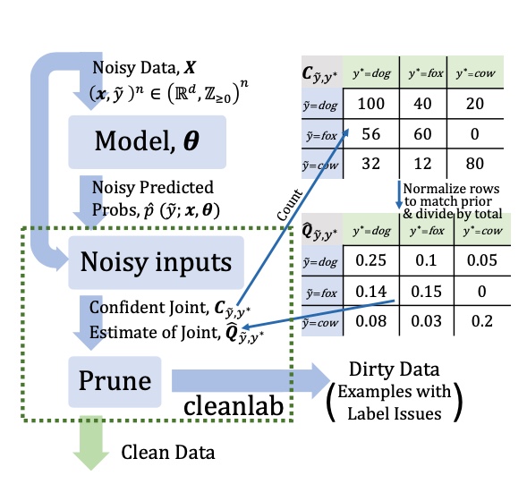
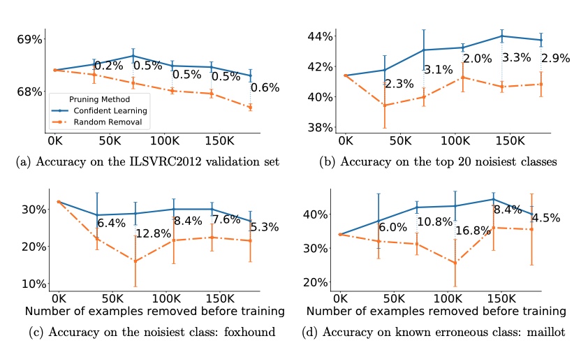
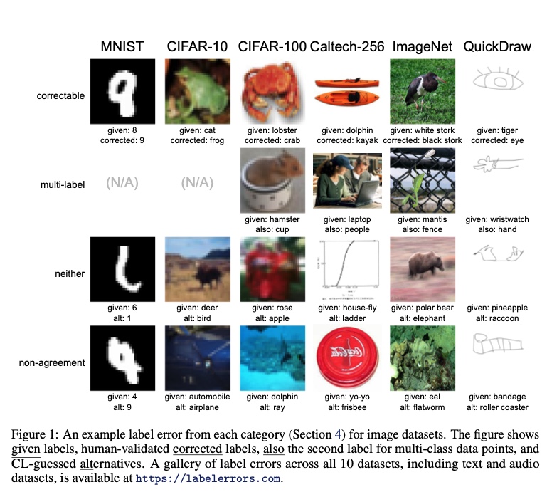
Examples of samples corrected using
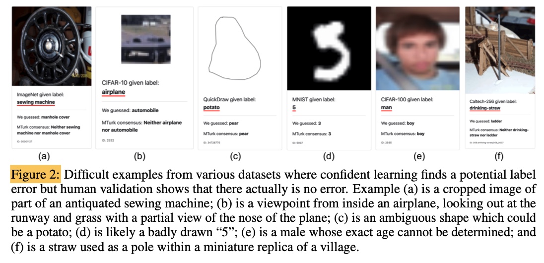
 Confident learning2.

CL is not 100% accurate. At the best, it is an effort to estimate noise using an epistemic uncertainty predictor [the model]. Having said that these examples it fails on are quite challenging as well.

Examples of samples Confident learning struggled with!2

Fundamentals

Let's look at the fundamentals CL builds on and dig in a bit on the antecedent and related works that formulate the foundation upon which Confident learning(cleanlab) is built!

  1. As discussed above already, is class conditional noise proposed by Angluin & Laird is the main concept utilized by CL.

  2. The use of weighted loss functions to estimate the probability of misclassification, as used in 7, is quite relevant to the field of CL, although it's not directly used in the CL technique as proposed by the Confident learning framework paper.

  3. Use of iterative noise cross-validation [INCV] techniques, as proposed in Chen et. al[8], that utilize a model-in-the-loop approach to finding noisy samples. This algorithm is shown below:

    Chen's INCV algorithm

  4. CL does not directly use MentorNet[6]. However, it is very relatable work that builds on a data-driven training approach. In simplistic terms, there is a teacher network that builds a curriculum of easy to hard samples (derived using loss measures) and the student is trained off this curriculum.

    MentorNet architecture

  5. There are other variations to data-driven teaching, one noticeable example is Co-teaching[9] which looks to be teaching each other in pairs and passing the non-noisy samples (calculated based on loss measures) to each other during learning. The main issue Co-teaching tries to solve is the memorization effects that are present in MentorNet[6]. (aka M-Net] but not in Co-teaching[9] due to data share.

    Co-teaching approach in contrast with MentorNet aka M-Net

  6. The understanding that small losses are a good indicator of useful samples and highly likely correct samples whereas jumpy, high loss producing samples are, well, interesting! They can be extreme edge cases or out-of-distribution samples or also can indicate wrongness. This only holds for reasonably performant models with abilities at least better than random chance if not more!

Limitations of CL

One thing that CL entirely ignores about label errors is when one or more true label is entirely missed. This is more likely to happen in multi-label settings and even more complex labeling setting like segmentation or detection than in multi-class classifications. For example, if there is a TV and water bottle in an image and the only annotation present is for the TV, and the water bottle is missed entirely! This is currently not modeled in CL as relies on building a pairwise class-conditional distribution between the given label and the true label. If the given label was a cat but the actual label was the dog for example. The framework itself does not allow it to model for the missing label when a true label is present.

Pairwise class-conditional distribution as proposed in CL also limits its use in multi-label settings. Explicitly when multiple labels can co-exist on the same data. For example, both the roof and swimming pool can be present in the image and they are not necessarily exclusive. This limitation comes from pairwise (single class gives vs single class predicted) modeling. This is different from say Stanford Car Dataset where make and model are predicted as multiple labels but they are exclusive ie a vehicle can be ute or hatchback but that is exclusive to it being made by Toyota or Volvo. Exclusivity in this case allows for modeling Pairwise class-conditional distribution. These are more multi-label multi-class modeled using multi-headed networks. True multi-label datasets can't be modeled like these pairwise joint distributions. They can perhaps be modeled using more complex joint distribution formulations but that would not scale very well. Confident learning[1] as it stands currently is a computationally expensive algorithm with an order of complexity being O(m2 + nm).

Having said these, it is probably something that is not explained in the literature as it seems that cleanlab itself supports multi-label classification. Conceptually I am unclear how multi-label works given the said theory. The support for multi-label is developing as issues are being addressed on this tool 1,2.

Hands on of label noise analysis using cleanlab for multi-label classification

Now that we have covered the background and theoretical foundations, let's try the confident learning out in detecting label noise using its implementation cleanlab. Specifically, I will use multi-label classification given the uncertainty around it (as discussed above)!. For this hands-on, I will use MLRSNet dataset. This spike is built using ResNet as a multi-label image classifier predicting 6 classes that can co-exist at the same time. These classes are ['airplane', 'airport', 'buildings', 'cars', 'runway', 'trees'] and derived off MLRSNet subset - i.e. only using airplane and airport.

The source code and this notebook for this project is label-noise Github repository. The notebook checks how well cleanlab performs in detecting label noise and identifies out-of-distribution samples, weird samples, and also errors!

Model info

Train and validation loss from the model trained using label-noise for 19 epochs. Note, for this spike, I opted out of n-fold cross-validation (CV). Using CV can lead to better results but its a not quick.

Training logs for the model used in this exercise (Image provided by author)

Exploration in noise using cleanlab

As shown in this notebook, the filter approach provided a list of samples that were deemed noisy. This flagged 38% of out-of-samples as noisy/erroneous.

Ranking provided an order in the samples on a 0-1 scale for label quality, the higher the number, the better quality the sample. I looked in get_self_confidence_for_each_label approach for out-of-distribution (OOD) samples and also entropy-based ordering. The distribution for each is as follows:

Confidance order of entropy-based ordering

Confidance order of self_confidence ordering

The samples picked as lowest quality or confidence is indeed rightfully chosen. There is an airplane that was missed in the image (shown in the highlighted overlay) and also another sample is OOD!

What's more interesting is all three methods of filtering, ranked by self-confidence and entropy all flagged these two samples! So we increase the threshold, and while there are false positives (for noise) there is some good example of errors.

False Positive True Positive

I am not sure if I am following how to interpret the pair-wise count for multi-label, so that's left for another day!

Conclusion

As discussed in this post, there are several reasons why label errors are unavoidable. While no small-efforts are required to minimize the errors in the dataset, management of the errors in the dataset is also warranted. The management to find noisy data, out of distribution data, or data that represents a systematic flaw (software/tooling issues or issues in the understanding of a concept that defines the target class). Approaches like model-in-loop, or additional information like ontology to find such noises or errors in the dataset are effective techniques. Confident learning provides a solid foundation for analyzing a dataset of noisy or OOD samples — a technique that’s quite effective for multi-class approaches, with the evolving support for multi-label classification. Now, on to cleaning the dataset! Happy cleaning!

References

  1. C. G. Northcutt, L. Jiang, and I. Chuang. Confident learning: Estimating uncertainty in dataset labels. Journal of Artificial Intelligence Research, 70:1373–1411, 2021. 1911.00068
  2. Northcutt, C. G., Athalye, A., and Mueller, J. (2021). Pervasive label errors in test sets destabilize machine learning benchmarks. In International Conference on Learning Representations Workshop Track (ICLR). 2103.14749
  3. D. Angluin and P. Laird. Learning from noisy examples. Machine Learning, 2(4):343–370, 1988. link
  4. Crowley RS, Legowski E, Medvedeva O, Reitmeyer K, Tseytlin E, Castine M, Jukic D, Mello-Thoms C. Automated detection of heuristics and biases among pathologists in a computer-based system. Adv Health Sci Educ Theory Pract. 2013 Aug;18(3):343-63. doi: 10.1007/s10459-012-9374-z. Epub 2012 May 23. PMID: 22618855; PMCID: PMC3728442. link
  5. Huan Ling and Jun Gao and Amlan Kar and Wenzheng Chen and Sanja Fidler, Fast Interactive Object Annotation with Curve-GCN. CVPR, 2019 link
  6. Jiang, L., Zhou, Z., Leung, T., Li, L.-J., and Fei-Fei, L. (2018). Mentornet: Learning data-driven curriculum for very deep neural networks on corrupted labels. In International Conference on Machine Learning (ICML).1712.05055.
  7. N. Natarajan, I. S. Dhillon, P. K. Ravikumar, and A. Tewari. Learning with noisy labels. In Conference on Neural Information Processing Systems (NeurIPS), pages 1196–1204, 2013. NurIPS 2013
  8. P. Chen, B. B. Liao, G. Chen, and S. Zhang. Understanding and utilizing deep neural networks trained with noisy labels. In International Conference on Machine Learning (ICML), 2019.1905.05040
  9. Han, B., Yao, Q., Yu, X., Niu, G., Xu, M., Hu, W., Tsang, I., and Sugiyama, M. (2018). Co-teaching: Robust training of deep neural networks with extremely noisy labels. In Conference on Neural Information Processing Systems (NeurIPS). 1804.06872

Review of recent advances in dealing with data size challenges in Deep Learning

The energy and excitement in machine learning and deep learning communities are infectious these days. So many groundbreaking advances are happening in this area but I have often found myself wondering why the only thing that makes it all shine - yes I am talking about the dark horse of deep learning the data is so underappreciated. The last few years of DL research have given me much joy and excitement and I carry hope now that going forward we can see some exciting progress in this space that explore advances in deep learning in conjunction with data! In this article, I summarise some of the recent developments in the deep learning space that I have been blown away by.

Table of content of this article: - Review of recent advances in dealing with data size challenges in Deep Learning - The dark horse of deep learning: data - Labelled data: the types of labels - Commonly used DL techniques centered around data - Data Augmentation - Transfer Learning - Dimensionality reduction - Active learning - Challenges in scaling dataset for deep-learning - Recent advances in data-related techniques - 1. Regularization - 1.1 Mixup - 1.2 Label Smoothing - 2. Compression - 2.1. X-shot learning: How many are enough? - 2.2. Pruning - 2.2.1 Coresets - 2.2.2 Example forgetting - 2.2.3 Using Gradient norms - 2.3. Distillation - 3. So what if you have noisy data - Conclusion - References

The dark horse of deep learning: data

Deep learning (DL) algorithms learn to perform a task by building a (domain) knowledge representation by looking at the training data. An early study of image models (classification and segmentation, year 2017) noted that the performance of the model increases logarithmically as the training dataset increases 1. The belief that increasing training dataset size will continue to increase model performance has been long-held. This has also been supported by another empirical study that validated this belief across machine translation, language modeling, image classification, and speech recognition 2 (see figure 1).

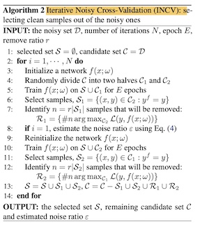
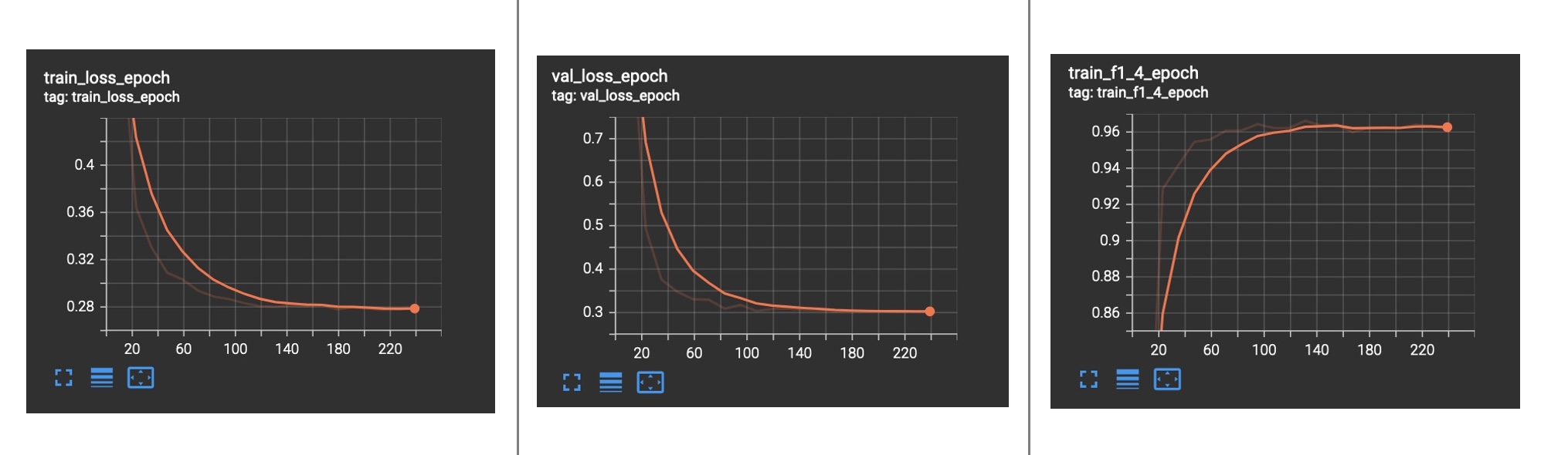
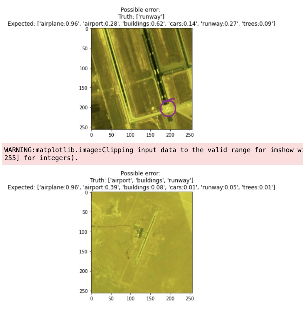
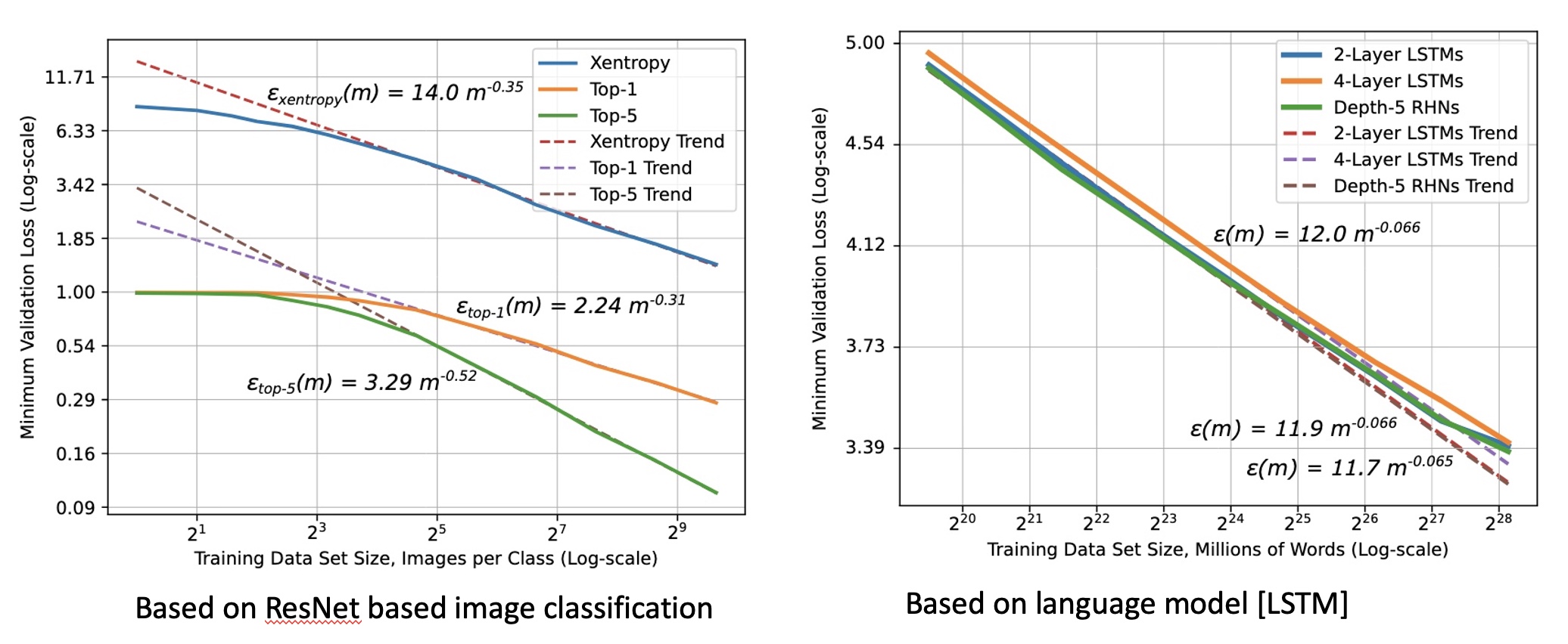
*Figure 1: Shows relationship between generalization error and dataset size (log scale) 2 *

So, the bigger dataset is better right? Almost! A theoretical foundation has been laid out in the form of power-law i.e $ \begin{equation} \label{power_law} ε(m) \approx αm^{β_g} \end{equation} $ wherein ε is generalization error, m is the number of samples in the training set, α is a constant property of the problem/DL task, and βg is the scaling exponent that defines the steepness of the learning curve. Here, βg, the steepness of the curve depicts how well a model can learn from adding more data to the training set 2 .(see figure 2) Empirically, βg was found to be between −0.07 and −0.35 despite theory suggesting βg to be 0.5 or 1. Nonetheless, the logarithmic relationship holds. As shown in figure 2, the gain eventually tapers in irreducible error.

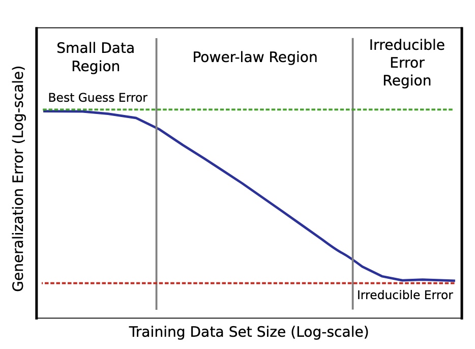
*Figure 2: Power Law curve showing model trained with a small dataset only as good as random guesses to rapidly getting better as dataset size increases to eventually settling into irreducible error region explained by a combination of factors including imperfect data that cause imperfect generalization 2 *

This can be attributed to several factors including imperfection in data. The importance of data quality and continually iterating over is touched on in some of the previous talks 1, 2, 3. Data quality matters, and so does the data distribution. The better the distribution of the training dataset is, the more generalized the model can be!


Data is certainly the new oil! 3


So, can we scale the data size without many grievances? Keep in mind, 61% of AI practicing organizations already find data and data-related challenges as their top challenge 4. If the challenges around procurement, storage, data quality, and distribution/demographic of the dataset has not subsumed you yet, this post focuses on yet another series of questioning. How can we train efficiently when data volume grows and the computation cost and turnaround time increase linearly with data growth? Then we begin asking how much of the data is superfluous, which examples are more impactful, and how do we find them? These are very important questions to ask given a recent survey 4 noted that about 40% of the organizations practicing AI already spend at least $1M per annum on GPUs and AI-related compute infrastructures. This should concern us all. Not every organization beyond the FAANG (and also, the one's assumed in FAANG but missed out on acronym!) and ones with big fat balance sheet will be able to leverage the gain by simply scaling the dataset. Besides, this should concern us all for environmental reasons and carbon emissions implications more details.

The carbon footprint of training a single AI is as much as 284 tonnes of carbon dioxide equivalent — five times the lifetime emissions of an average car source.

The utopian state of simply scaling training datasets and counting your blessings simply does not exist. The question then is, what are we doing about it? Unfortunately not a whole lot especially if you look at the excitement in the ML research community in utilizing gazillion GPU years to gain a minuscule increase in model performance attributed to algorithmic or architectural changes. But the good news is this area is gaining much more traction now. Few pieces of research since 2020 are very promising albeit in their infancy. I have been following the literature around the use of data in AI (a.k.a data-centric AI) topic very closely as this is one of my active areas of interest. I am excited about some of the recent developments in this area. In this post, I will cover some of my learnings and excitement around this topic.

Before, covering them in detail, let's review foundational understanding and priors first:

Labelled data: the types of labels

This post focuses heavily on supervised learning scenarios focussing mainly on computer vision. In this space, there are two types of labels: - Hard labels - Soft labels

Traditional labels are hard labels where the value of ground truth is a discrete value e.g. 0 and 1, 0 for no, and 1 for yes. These discrete values can be anything depending on how the dataset was curated. It's important to note that these values are absolute and unambiguously indicate their meaning.

There is an emerging form of labels known as soft labels where ground through represents the likelihood. By nature these labels are continuous. An example, a pixel is 40% cat 60% dog. It will make a whole lot of sense in the following sections.

Commonly used DL techniques centered around data

Data augmentation and transfer learning are two commonly used techniques in deep learning these days that focus on applying data efficiently. Both these techniques are heavily democratized now and commonly applied unless explicitly omitted.

Data Augmentation

Data augmentation encompasses a variety of techniques to transform a datapoint such that it adds variety to the dataset. The technique aims to keep the data distribution about the same but add richness to the dataset by adding variety. Predominantly, the transformation via this technique has been intra-sample. Affine transformations, contrast adjustment, jittering, or color balancing are some such examples of data augmentation techniques. Imgaug and kornia are very good libraries for such operation even though all ML frameworks offer a limited set of data augmentation routines.

Data augmentation technique was initially proposed to increase robustness and achieve better generalization in the model but they are also used as a technique to synthetically increase data size as well. This is especially true in cases where data procurement is really challenging. These days, data augmentation techniques have become a lot more complex and richer including scenarios where-in model-driven augmentations may also be applied. One example of this is GAN-based techniques to augment and synthesize samples. In fact, data augmentation is also one of the techniques to build robustness against adversarial attacks.

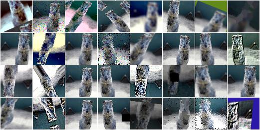
* Example of augmentation src *

Transfer Learning

Transfer learning is a very well democratized technique as well that stems from reusing the learned representations into a new task if the problem domain of two tasks is related. Transfer learning relaxes the assumption that the training data must be independent and identically distributed (i.i.d.) with the test data 5, allowing one to solve the problem of insufficient training data by bootstrapping model weights from another learned model trained with another dataset.

*Figure 3: Training with and without transfer learning 6 *

With transfer learning, faster convergence can be achieved if there is an overlap between the tasks of the source and target model.

Dimensionality reduction

Dimension reduction techniques are also applied to large datasets:

These techniques are categorized into two: 1. Ones that seek to preserve the pairwise distance amongst all the samples in the dataset. Principal component analysis (PCA) is a good example of this. 2. Ones that preserve the local distances over global distance. The techniques like uniform manifold approximation and projection (UMAP) 23 and t-distributed stochastic neighbor embedding (t-SNE) 24 fit in this category. UMAP arguably preserves more of the global structure and is algorithmically faster than t-sne. Both T-SNE and UMAP use gradient descent for arriving at the optimal embeddings.

These techniques in DL space however are mostly used to understand the data and also for visualization purposes. UMAP and T-SNE do better at preserving global structure than other embedding algorithms but are limited. This blog covers the topic more in detail.

Active learning

Active learning is a methodology wherein the training process proactively asks for labels on specific data. It is used more commonly in classical ML techniques, but it has not been very successful in deep learning due to back-propagation. Offline or pool-based active learning has been investigated heavily for use in deep learning but without much groundbreaking success. The use of active learning is not very straightforward either due to the negative impact of outliers on training 25. Pool-based active learning will be covered in the following section in more detail (pruning).

Challenges in scaling dataset for deep-learning

Besides the techniques discussed in previous section, not a lot of investment has been done in the area focussing on data-centric AI. The momentum around data-centric AI is forming a bit recently with Andrew Ng driving data-centric AI efforts through his new startup Landing.AI.

In my view, the following are some of the broad categories of questions that fall under the purview of data-centric AI:

  1. How to efficiently train with the rapid increase in the dataset? Yann LeCun called out in his interview with Soumith Chintala during PyTorch developer day 2021 that training time of more than 1 week should not be acceptable. This is a very good baseline for practical reasons but if one does not have an enormous GPU fleet at their disposal then this is goalpost is very hard to achieve given current DL practices. So, what else can be done to train efficiently with increased dataset size?
  2. Are all samples equally important? How important a sample in the dataset is? Can we leverage the "importance factor" for good?
  3. What role does a sample play towards better generalization? Some samples carry redundant features, so how to deduplicate the dataset when features as in DL are not explicit?
  4. Data size matters but can we be strategic about what goes in the dataset?
    1. Cleverly doing this has to do with efficient sampling and data mining techniques. These are the easily solved problem if and only if we know what our targets are. Challenge in DL, as I see it, is what to look for to mine for the best sample? This is not well understood.
  5. How can we leverage more innate DL techniques like objective functions, backpropagation, and gradient descent to build a slick and effective dataset that provides the highest return on investment.
  6. Noises in datasets are seen as evil. But are they always evil? How much noise can one live with? How to quantify this?
  7. How much of a crime it is if data bleeds across traditional train/validate/calibrate/test splits.
    1. What are the recommendations on the data split for cascade training scenarios?
  8. How fancy can one get with data augmentation before returns start to diminish?
  9. How to optimize the use of data if continual learning is observed?

If we look at humans are learning machines, they have infinite data at their disposal to learn from. Our system had evolved into efficient strategies to parse through infinite data streams to select the samples we are interested in. How our vision system performs foveal fixation utilizing saccadic eye movements to conduct efficient subsampling of interesting and useful datapoint should be a good motivation. Sure we fail sometimes, we fail to see the pen on the table even though it's right in front of us due to various reasons but we hit it right most of the time. Some concepts of Gestalt theory, a principle used to explain how people perceive visual components (as organized patterns, instead of many disparate parts) are already applicable for better selection of data even if machine models are stochastic parrots. According to this theory, eight main factors, listed below, determine how the visual system automatically groups elements into patterns.

  1. Proximity: Tendency to perceive objects or shapes that are close to one another as forming a group.
  2. Similarity: Tendency to group objects if physical resemblance e.g. shape, pattern, color, etc. is present.
  3. Closure: Tendency to see complete figures/forms even if what is present in the image is incomplete.
  4. Symmetry: Tendency to ‘see’ objects as symmetrical and forming around a center point. 50
  5. Common fate: Tendency to associate similar movement as part of a common motion.
  6. Continuity: Tendency to perceive each object as a single uninterrupted i.e. continuous object
  7. Good Gestalt: Tendency to group together if a regular, simple, and orderly pattern can be formed
  8. Past experience: Tendency to categorize objects according to past experience.

Of these, I argue, proximity, similarity, common fate, and past experience are relevant. I even argue on the possibility of applying closure. A recent work by FAIR 22, shows that machine models can fill in the gaps and infer missing pieces correctly by applying minor changes commonly used technique autoencoders. Why I bring this up with so much excitement than GAN-based techniques of hallucination is how easy it is to build and train as compared to GAN.

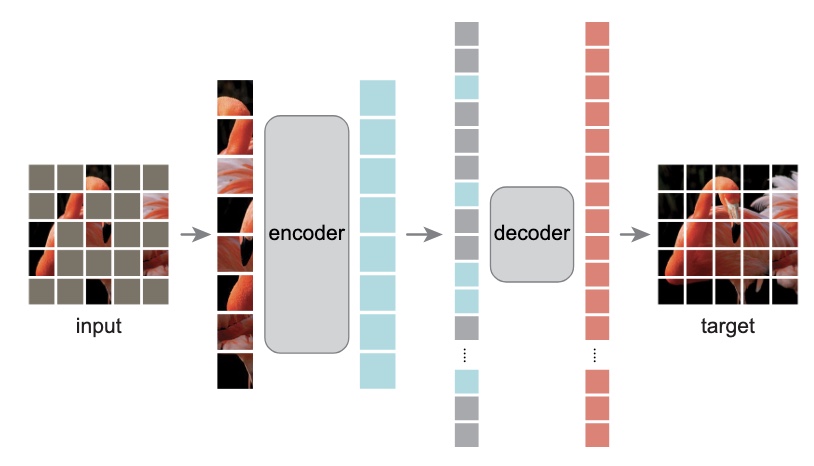
Masked-Autoencoders showing model inferring missing patches 22

Its been interesting to note that the recent advances towards dealing with the challenges of scaled data are largely inspired by already known deep-learning techniques except they are now applied through the lens of data. Examples like pruning, compression, sampling strategies, and leveraging from phenomena such as catastrophic forgetting, knowledge distillation.

Technique How it's presently utilized in model building Proposed data-centric view
Prunning A specialized class of model compression technique where low magnitude weights are eliminated to reduce the size and computational overhead. Samples that don't contribute much to generalization are omitted from the training regime.
Compression A broad range of model compression techniques to reduce the size and computational overhead includes techniques like quantization wherein some amount of information loss is expected. A broad range of data filtering and compression techniques to reduce size without compromising much on generalization.
Distillation To extract learned representation from a more complex model to a potentially smaller model. To extract knowledge present in the larger dataset into a smaller synthesized set.
Loss function Also termed as the objective function is the one of core concepts of DL that defines the problem statement. As shown in 22, and also more broadly can be leveraged to fill in missing information in the data.
Regularisation One of the theoretical principles of DL is applied through various techniques like BatchNorm, Dropouts to avoid overfitting. Variety of techniques to ensure overfitting applied with data in mind, e.g. Label Smoothing 7,10

*Table 1: Summary of techniques that are crossbreed from core DL techniques to also into data-centric DL *

Let's dive into the details of how these classes of techniques are applied through the lens of data:

1. Regularization

1.1 Mixup

Mixup is a special form of data augmentation technique that looks beyond intra-sample modification and explores inter-sample modification. The idea with mixup is to linearly combine (through convex geometry) a pair of samples to result into one.

$ \begin{equation} x\prime=λx_i + (1−λ)x_j , \ \text{where,} λ ∈ [0,1] \ \text{ drawn from beta distribution, and xi, xj are input/source vector} \end{equation} $

$ \begin{equation} y\prime = λy_i + (1 − λ)y_j , \ \text{where y_i , yj are one-hot label encodings} \end{equation} $

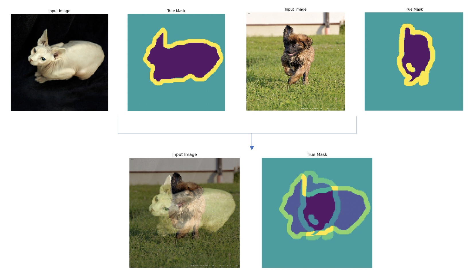
*Figure 4: Sample produced by applying mixup 7 on Oxford Pets dataset *

Mixup 7 in fact seeks to regularize the neural network to favor simple linear behavior in-between training examples. As shown in fig 5, mixup results in better models with fewer missed. Its been shown that mixup increases the generalization, reduces the memorization of corrupt labels, increases the robustness towards adversarial examples 7,8.

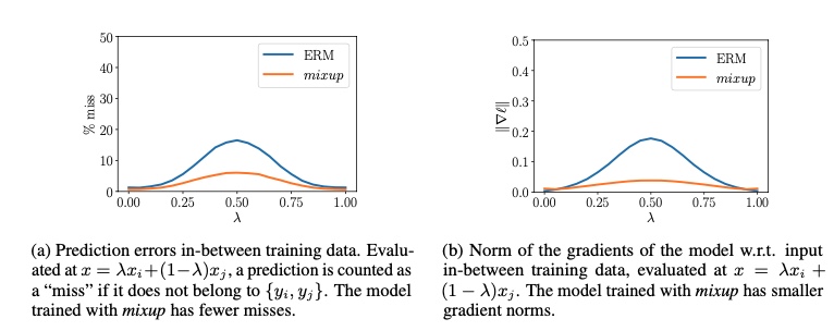
Figure 5: Shows that using mixup 7, lower prediction error and smaller gradient norms are observed.

I see mixup as not only an augmentation, and regularisation technique but also a data compression technique. Depending on how frequently (say α) the mixup is applied, the dataset compression ratio (Cr) will :

$ \begin{equation} C_r = 1 - α/2 \end{equation} $

If you have not noticed already, applying mixup convert labels to soft labels. The linear combination of discreet values will result in a continuous label value that can explain the example previously discussed wherein the pixel is 40% cat 60% dog (see fig 5).

1.2 Label Smoothing

Label smoothing 10 is a form of regularisation technique that smoothes out ground truth by a very small value epsilon ɛ. One motivation for this is of course better generalization and avoiding overfitting. While the other motivation is to discourage the model from becoming overconfident. Both 8,10 have shown that label smoothing leads to better models.

$ \begin{equation} Q_{i} = \begin{cases} \displaystyle 1 - ɛ & \text{if i == k,} \
ɛ/K & \text{Otherwise, where K is number of classes} \
\end{cases}
\end{equation} $

Label smoothing as indicated by the equation above does not lead to any visible differences in label data as ɛ is really small. However, applying mixup change visibly changes both source (x) and the label (y).

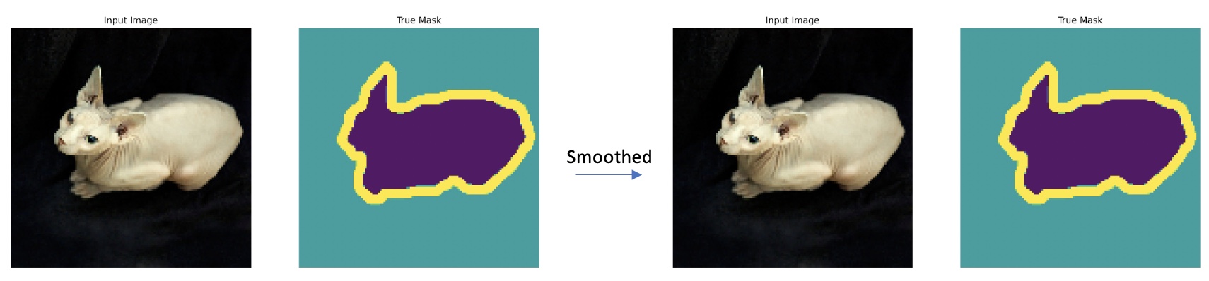
Applying label-smoothing has no noticeable difference

2. Compression

Compression refers to a broad range of data filtering and compression techniques to reduce size without compromising much on generalization. Following are some of the recent exciting development on this front:

2.1. X-shot learning: How many are enough?

The troubles of high computational cost and long training times due to an increase in the dataset have led to the development of training by a few shot strategies. The intuition behind this approach is to take a model and guide it to learn to perform a new task only by looking at a few samples 11. The concept of transfer learning is implicitly applied in this approach. This line of investigation started with training new tasks by using only a few (handful) samples and explored an extreme case of one-shot training i.e. learning new tasks from only one sample 12,13.

Recently an interesting mega-extreme approach of shot-based learning has emerged - ‘Less Than One’-Shot Learning a.k.a LO Shot learning 11. This approach utilizes soft label concepts and seeks to merge hard label N class samples into M samples where M < N and thus the name less than one! LO Shot-based techniques are a form of data compression technique and may feel very similar to the MixUp technique discussed earlier. However, LO Shot contrary to a convex combination of samples as in Mixup, exploits distance weighted k-Nearest Neighbours technique to infer the soft labels. Their algorithm termed distance-weighted soft-label prototype k-Nearest Neighbours (SLaPkNN) essentially takes the sum of the label vectors of the k-nearest prototypes to target point x, with each prototype weighted inversely proportional to its distance from x. The following figure shows 4 class datasets are merged into 2 samples using SLaPkNN.

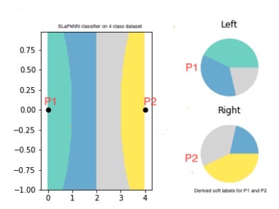
Figure LO-Shot: LO Shot splitting 4 class space into 2 points 11.

In my understanding that is the main theoretical difference between the two techniques, with the other difference being mixup only merges two samples into one using a probability drawn from beta distribution combined using λ and 1-λ whereas LO is more versatile and can compress greatly. I am not saying mixup cant be extended to be more multivariate but that empirical analysis of such approach is unknown; whereas with 11 its been shown SLaPkNN can compress 3M − 2 classes into M samples at least.

The technical explanation for this along with code is available here.

2.2. Pruning

Pruning is a subclass of compression techniques wherein samples that are not really helpful or effective are dropped out whereas selected samples are kept as is without any loss in content. Following are some of the known techniques of dataset pruning:

2.2.1 Coresets

Coreset selection technique pertains to subsampling from a large dataset to a smaller set that almost approximates the given large set. This is not a new technique and has heavily been explored using hand-engineered features and simpler models like Markov models to approximate the smaller set. This is not a DL-specific technique either and has its place in classical ML as well. An example could be using naïve Bayes to select coresets for more computationally expensive counterparts like decision trees.

In deep learning, using a similar concept, a lighter-weight DL model can be used as a proxy to select the approximate dataset 15. This is easier achieved when continual learning is practiced otherwise it can be a very expensive technique in itself given proxy model needs to be trained with a full dataset first. This becomes especially tricky given the proxy and target models are different and also when the information in the dataset is not concentrated in a few samples but uniformly distributed over all of them. These are some of the reasons why this approach is not very successful.

2.2.2 Example forgetting

An investigation 14 reported that some samples once learned are never forgotten and exhibit the same behavior across various training parameters and hyperparameters. There are other classes of samples that are forgotten. The forgetting event was defined as when the model prediction regresses in the subsequent epoch. Both qualitative and qualitative (see fig 6 and 7) analysis into such forgotten samples indicated noisy labels, images with “uncommon” visually complicated features were the main reasons for example forgetting.

w 
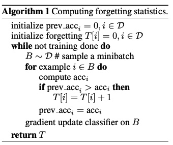
Figure 6: Algorithm to track forgotten samples 14.

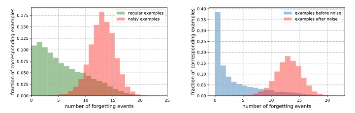
Figure 7: Indicating how increasing fraction of noisy samples led to increased forgetting events 14.

An interesting observation from this study was that losing a large fraction of unforgotten samples still results in extremely competitive performance on the test set. The hypothesis formed was unforgotten samples are not very informative whereas forgotten samples are more informative and useful for training. In their case, the forgetting score stabilized after 75 epochs (using RESNET & CIFAR but the value will vary as per model and data).

Perhaps a few samples are enough to tell that a cat has 4 legs, a small face, and pointy ears, and it's more about how different varieties of cats look especially if they look different from the norm e.g. Sphynx cats.

2.2.3 Using Gradient norms

Loss functions are an excellent measure to find interesting samples in your dataset whether these may be poorly labeled or really outlier samples. This was highlighted by Andrej Karpathy as well:

When you sort your dataset descending by loss you are guaranteed to find something unexpected, strange, and helpful.

Personally, I have found loss a very good measure to find poorly labeled samples. So, the natural question would be "should we explore how we can use the loss as a measure to prune the dataset?". It's not until NeurIPS 2021, 21 that this was properly investigated. This Standford study looked into the initial loss gradient norm of individual training examples, averaged over several weight initializations, to prune the dataset for better generalization. This work is closely related to example forgetting except that instead of performance measure the focus more is on using local information early in training to prune the dataset.

This work proposes GraNd score of a training sample (x, y) at time t given by L2 norm of the gradient of loss computed on that sample and also expected loss L2 norm termed EL2N (equation below). The reasoning here is that samples with a small GraNd score have abounded influence on learning how to classify the rest of the training data at a given training time. Empirically, this paper found that averaging the norms over multiple weight initializations resulted in scores that correlate with forgetting scores 14 and leads to pruning a significant fraction of samples early in training. They were able to prune 50% of the sample from CIFAR-10 without affecting accuracy, while on the more challenging CIFAR-100 dataset, they pruned 25% of examples with only a 1% drop in accuracy.
$ \begin{equation} χ_t(x, y) = E_{w_t} || g_t(x, y)||_2 \ \tag*{GraNd eq} \ \end{equation} $

$ \begin{equation} χ_t(x, y) = E || p(w_t, x) - y)||_2 \ \tag*{EL2N eq} \ \end{equation} $

This is a particularly interesting approach and is a big departure from other pruning strategies to date which treated samples in the dataset independently. Dropping samples based on independent statistics provides a weaker theoretical guarantee of success as DL is a non-convex problem 21. I am very curious to find out how mixup impacts the GraNd scores given it shown (see figure 5b) using mixup leads to smaller gradient norm (l1 albeit).

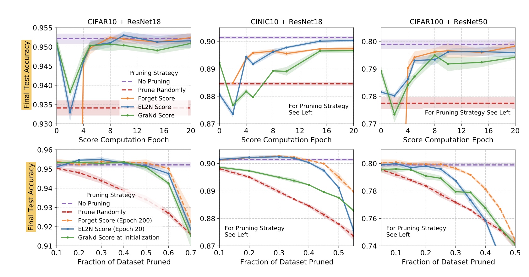
Results of prunning with GradNd and EL2N 21.

The results from this study are shown in the fig above. Noticeably high pruning is not fruititious even with this approach despite how well it's doing on CIFAR-10 and 100 datasets. Are we retaining the data distribution when we drop large samples? Mostly not and that is only reasoning that makes sense. And we circle back to how much pruning is enough? Is that network dependent or more a property of data and its distribution? This study 21 claims that GradND and EL2N scores, when averaged over multiple initializations or training trajectories remove dependence on specific weights/networks, presenting a more compressed dataset. If this assertion holds in reality, in my view, this is a very promising finding easing the data-related challenges of DL.

What's more fascinating about this work is that it sheds light on how the underlying data distribution shapes the training dynamics. This has been amiss until now. Of particular interest is identifying subspaces of the model’s data representation that are relatively stable over the training.

2.3. Distillation

Distillation technique refers to the methodologies of distilling the knowledge of a complex or larger set into a smaller set. Knowledge or model distillation is a popular technique that compresses the learned representation of a larger model into a much smaller model without any significant drop in performance. Using student-teacher training regime have been explored extensively even in the case of transformer networks that are even more data-hungry than more conventional network say Convolution network DeiT. Despite being called data-efficient, this paper employs a teacher-student strategy to transform networks, and data itself is merely treated as a commodity.

Recently, this concept is investigated for use in deep learning for dataset distillation with aim of synthesizing an optimal smaller dataset from a large dataset 17,16. The distilled dataset are learned and synthesized but in theory, they approximate the larger dataset. Note that the synthesized data may not follow the same data distribution.

Some dataset distillation techniques refer to their approach as compression as well. I disagree with this in principle as compression albeit lossy in this context, refers to compressing the dataset whereas with distillation the data representation is deduced/synthesized - potentially leading to entirely different samples together. Perhaps it's the compressibility factor a.k.a compression ratio that applies to both techniques. For example, see figure 13 shows the extent to which distilled images can change.

A dataset distillation 17 paper quotes:

We present a new optimization algorithm for synthesizing a small number of synthetic data samples not only capturing much of the original training data but also tailored explicitly for fast model training in only a few gradient steps 17.

Their problem formulation was very interesting! they derive the network weights as a differentiable function of the synthetic training data and set the training objective to optimize the pixel values of the distilled images The result from this study showed that one can go as low as one synthetic image per category while not regressing too much on the performance. More concretely, they distilled 60K training images of the MNIST digit dataset into only 10 synthetic images (one per class) yields a test-time MNIST recognition performance of 94%, compared to 99% for the original dataset).

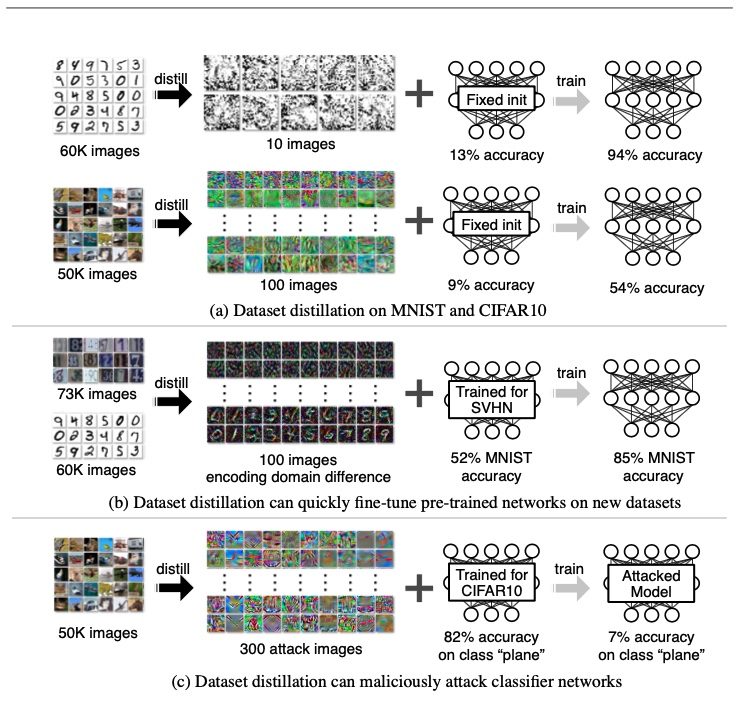
Figure 8: Dataset distillation results from FAIR study 17.

Here are some of the distilled samples for the classes labeled at the top (fig 9). It's amazing how well the MNIST trained on these sets does but CIFAR one misses the mark only being about as good as random (54%) compared to 80% on the full dataset(fig 8 & 9).

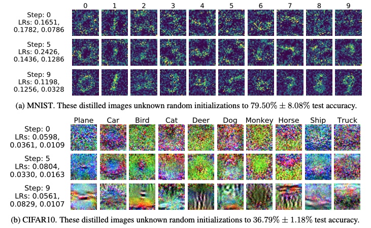
Figure 9: Dataset distillation results from FAIR study 17.

Following this work, another distillation technique was proposed utilizing kernel methods - more specifically kernel ridge regression to obtain ε-approximate of original datasets 18. This technique is termed Kernel Inducing Points (KIP) and follows the same principle for keeping the objective function to maximize the approximation and backpropagate the gradients to learn synthesized distilled data. The difference between 18 and 17 is one 17 uses the same DL network while the other 18 uses kernel techniques. With KIP, another advantage is that not just source samples but optionally labels can be synthesized too. In 17, the objective was purely to learn pixel values and thus the source (X). This paper 18 also proposes another technique Label Solve (LS) in while X is kept constant and only label (Y) is learned.

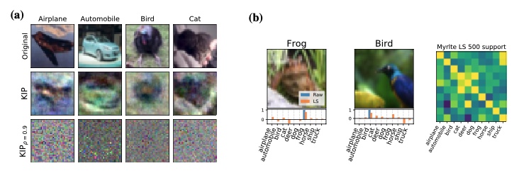
Figure 10: Examples of distilled samples a) with KIP and b) With LS 18.

The CIFAR 10 result from 17 (fig 9) was about 36.79% for 10 samples, with KIP there is a slight gain in performance there given the extreme compression. This raises the question of what is a good compression ratio that can guarantee good information retention. For complex tasks like CIFAR (compared to MNIST), 10 (one per sample) may not be enough given how complex this dataset is comparatively.

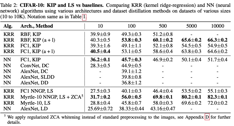
Figure 11: CIFAR10 result from KIP and LS 18.

Actually, LO shot technique 11, discussed previously, is also a specialized form of X-shot technique that does dataset distillation. Aside from that, gradient-based techniques for dataset distillation have been actively investigated in the last few years (ref 16,17,18,19,20). Another approach explored siamese augmentation method termed Differentiable Siamese Augmentation (DSA) that uses matching loss and synthesizes dataset through backpropagation techniques 16

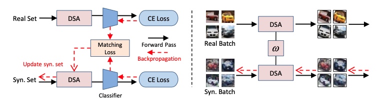
Figure 12: Differentiable Siamese Augmentation 16.

Bayesian and gradient-descent trained neural networks converge to Gaussian processes (GP) as the number of hidden units in intermediary layers approaches infinity 20 (fig 13). This is true for convolutional networks as well as they converge to a particular gaussian processes channel limits are stretched to infinity. These networks can thus be described as kernels known as Neural Tangent Kernel (NTK). Neural Tangents library based on JAX an auto differentiation toolkit has been used in applying these kernels in defining some of the recent distillation methods. References 18,20,21 are one such examples.

Figure 13: Infinite width Convolution networks converging to infinity 20.

The authors of KIP and LS techniques 18 explore how to scale and accelerate the distillation process to apply these techniques to infinitely wide convolutional networks 20. Their results are very promising (see fig 14).

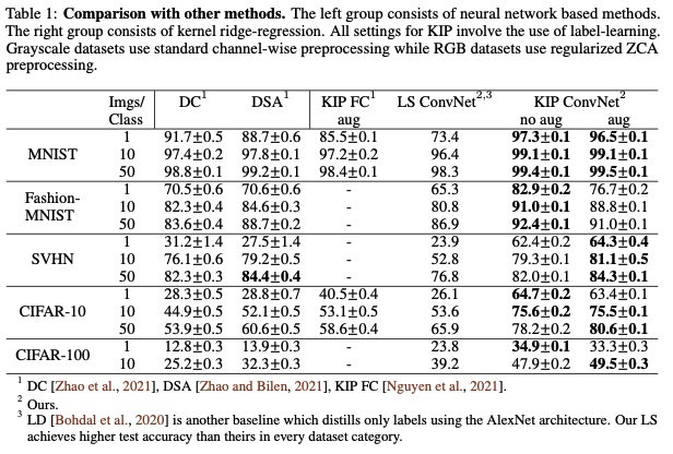
Figure 14: KIP ConvNet results 20.

A visual inspection into the distilled dataset from the infinite width CNN-based KIP technique is shown in fig 15. The distillation results are curious, to say the least. In the example, the distilled apple image seems to represent a pile of apples whereas the bottle distilled results into visibly different bottles while still showing artifacts of the original two bottles. While other classes show high order features (with some noise).

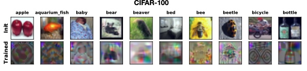
Figure 15: KIP ConvNet example of distilled CIFAR set 20.

Figure 16 shows MNIST results, they are not only very interesting but also look very much like mixup (where x and y both are mixed).

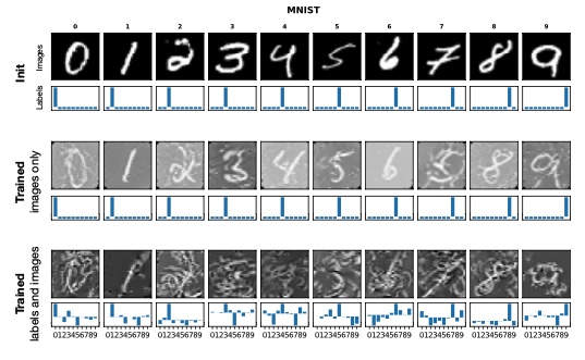
Figure 16: KIP ConvNet example of distilled MNIST set 20.

3. So what if you have noisy data

Noises in the dataset are considered a nuisance. Because models hold the compressed form of knowledge represented by the dataset, dataset curation techniques carefully look to avoid noises in datasets.

Noises can be an incredibly powerful technique to fill in the missing information in source/images. For instance, if only part of an image is known then instead of padding the image with default (0 or 1-pixel value), filling in using random noise can be an effective technique avoiding confusion on actual real values that relate to the black or white region. This has held true in my own experience. It was very amusing to note that the forgetting event study 14 in fact looked into adding label noise on the distribution of forgetting events. They added noise in pixel values and observed that adding an increasing amount of noise decreases the number of unforgettable samples (see also figure 7 for their results when noise was used).

Noise coming from randomness is handled very well by DL networks as well. I find the result from 22, shown in figure 17 quite fascinating actually. Looking at how well the model is doing when missing patches are random and how poor it is doing when missing patches are systematic is indicative of how powerful and lame (both at the same time) machines are!

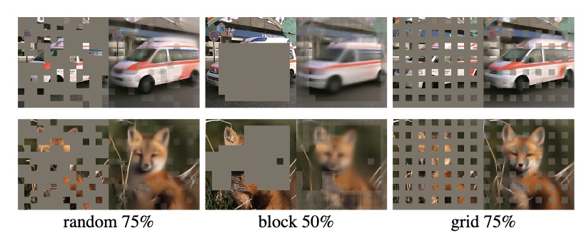
Figure 17: Noisy patches in Masked-AutoEncoder 22.

GradND study 21, looked into the effect of noise on the source itself and performed a series of experiments to conclude that when there is enough data, keeping the high score examples, which are often noisy or difficult, does not hurt performance and can only help.

Conclusion

In summary, the last four years have been incredibly exciting for data in DL space and the year 2021 even more! There is a lot of mileage we can get out of simpler techniques like MixUp but more exciting developments are dissecting the training dynamics and exploring the importance of samples in solving a particular task using DL techniques. Distillation methods are still in the early stages where they work well for simpler datasets but honestly how many real-world problems have simple datasets? Nevertheless, some really exciting development in this space. These techniques can be groundbreaking if the compression methods hold across a wide range of architectures as indicated by 21.

References

  1. [1707.02968] Revisiting Unreasonable Effectiveness of Data in Deep Learning Era.” Accessed January 3, 2022. https://arxiv.org/abs/1707.02968.
  2. Hestness, Joel, Sharan Narang, Newsha Ardalani, Gregory Diamos, Heewoo Jun, Hassan Kianinejad, Md Mostofa Ali Patwary, Yang Yang, and Yanqi Zhou. “Deep Learning Scaling Is Predictable, Empirically,” December 2017. https://arxiv.org/abs/1712.00409.
  3. https://www.wired.com/story/no-data-is-not-the-new-oil/
  4. https://pages.run.ai/hubfs/PDFs/2021-State-of-AI-Infrastructure-Survey.pdf
  5. [1808.01974] A Survey on Deep Transfer Learning. Accessed January 5, 2022. https://arxiv.org/abs/1808.01974.
  6. Transfer Learning. http://citeseerx.ist.psu.edu/viewdoc/download?doi=10.1.1.146.1515&rep=rep1&type=pdf
  7. Zhang, Hongyi, Moustapha Cisse, Yann N. Dauphin, and David Lopez-Paz. “Mixup: Beyond Empirical Risk Minimization,” October 2017. https://arxiv.org/abs/1710.09412.
  8. [1812.01187] Bag of Tricks for Image Classification with Convolutional Neural Networks. Accessed December 30, 2021. https://arxiv.org/abs/1812.01187.
  9. [2009.08449] ’Less Than One’-Shot Learning: Learning N Classes From M < N Samples. Accessed January 5, 2022. https://arxiv.org/abs/2009.08449.
  10. [1512.00567] Rethinking the Inception Architecture for Computer Vision. Accessed January 5, 2022. https://arxiv.org/abs/1512.00567.
  11. [1904.05046] Generalizing from a Few Examples: A Survey on Few-Shot Learning. Accessed January 5, 2022. https://arxiv.org/abs/1904.05046.
  12. Li Fei-Fei, R. Fergus and P. Perona, “One-shot learning of object categories,” in IEEE Transactions on Pattern Analysis and Machine Intelligence, vol. 28, no. 4, pp. 594–611, April 2006, doi: 10.1109/TPAMI.2006.79. https://ieeexplore.ieee.org/document/1597116
  13. [1606.04080] Matching Networks for One Shot Learning. Accessed January 5, 2022. https://arxiv.org/abs/1606.04080.
  14. [1812.05159] An Empirical Study of Example Forgetting during Deep Neural Network Learning. Accessed December 29, 2021. https://arxiv.org/abs/1812.05159.
  15. [1906.11829] Selection via Proxy: Efficient Data Selection for Deep Learning. Accessed December 29, 2021. https://arxiv.org/abs/1906.11829.
  16. [2102.08259] Dataset Condensation with Differentiable Siamese Augmentation. Accessed January 5, 2022. https://arxiv.org/abs/2102.08259.
  17. [1811.10959] Dataset Distillation. Accessed January 5, 2022. https://arxiv.org/abs/1811.10959.
  18. [2011.00050] Dataset Meta-Learning from Kernel Ridge-Regression. Accessed January 5, 2022. https://arxiv.org/abs/2011.00050.
  19. [2006.05929] Dataset Condensation with Gradient Matching. Accessed January 5, 2022. https://arxiv.org/abs/2006.05929.
  20. [2107.13034] Dataset Distillation with Infinitely Wide Convolutional Networks. Accessed January 5, 2022. https://arxiv.org/abs/2107.13034.
  21. [2107.07075] Deep Learning on a Data Diet: Finding Important Examples Early in Training. Accessed December 10, 2021. https://arxiv.org/abs/2107.07075.
  22. [2111.06377] Masked Autoencoders Are Scalable Vision Learners. Accessed January 5, 2022. https://arxiv.org/abs/2111.06377.
  23. [1802.03426] UMAP: Uniform Manifold Approximation and Projection for Dimension Reduction. Accessed January 5, 2022. 23. https://arxiv.org/abs/1802.03426.
  24. Maaten, Laurens van der and Geoffrey E. Hinton. “Visualizing Data using t-SNE.” Journal of Machine Learning Research 9 (2008): 2579–2605. https://www.jmlr.org/papers/volume9/vandermaaten08a/vandermaaten08a.pdf
  25. [2107.02331] Mind Your Outliers! Investigating the Negative Impact of Outliers on Active Learning for Visual Question Answering.” Accessed January 8, 2022. https://arxiv.org/abs/2107.02331