From Evaluation to Integration: How AI Became Ready for Children's Book Production
"Cliché, my dear parrot! Cliché!"
That was my assessment in January 2023, watching ChatGPT reach for the tired apple-falling-on-Newton's-head trope when I asked it to write a children's book about physics. The verdict was clear: the technology wasn't ready. Not because AI couldn't eventually augment creative work—that was always the obvious trajectory—but because the 2023 output quality was too poor for augmentation to be meaningful. You can't build on a foundation that produces intellectually shallow, pedagogically unsound content. Adding AI assistance to a broken core would only scale the problems.
Two years later, the calculus has changed. I've built FableFlow, an open-source agentic AI pipeline for children's book production, and repositioned the entire Curious Cassie series around AI-augmented storytelling.
This post examines what changed technically, what remains problematic, and what this evolution means for authors, publishers, and the broader question of AI in creative domains.
The 2023 Assessment: What Held Up and What Didn't
Re-reading my original piece provides a useful benchmark for how the technology has evolved.
Assessments That Held Up
1. Content Quality Was Insufficient ChatGPT in January 2023 produced narratives that were structurally competent but intellectually hollow. When prompted to write about Newton's discoveries, it delivered the apple cliché and surface-level explanations of the laws of motion. The content lacked what educators call "productive struggle"—the carefully calibrated cognitive challenges that build genuine understanding. This assessment was correct: using that output as a foundation for augmentation would have produced polished mediocrity at best.
2. Governance Gaps Remain I noted that society wasn't ready for AI-generated children's content. This has proven accurate. The past two years have seen an explosion of AI-generated children's books on content platforms — much of it low-quality, some containing hallucinated or inappropriate content that slipped past moderation. The governance frameworks remain inadequate, and the flood of AI-generated content has created signal-to-noise problems for parents and educators.
3. Cognitive Offloading Risk The concern about "depleting creative and critical thinking abilities in favour of convenience" remains valid. The ease of AI generation creates genuine risk of cognitive offloading—similar to how GPS navigation has measurably reduced spatial reasoning capabilities in regular users. This requires ongoing vigilance in how AI tools are designed and used.
Where the Analysis Was Incomplete
1. The Framing Was Too Narrow The original piece was titled "ChatGPT vs Me"—framing the question as whether AI could match human authorship. This was the wrong frame. The interesting question was never about replacement but about composition: what becomes possible when human creative vision is combined with AI production capability? In 2023, the answer was "not much, because the AI components aren't good enough." By 2025, that answer has changed substantially.
2. Underestimating Improvement Velocity The jump from GPT-3.5 to GPT-4 to Claude 3.5 to current frontier models isn't just quantitative—it's qualitative. Instruction-following, long-context coherence, and iterative refinement capabilities have crossed thresholds that enable genuine collaboration rather than simple generation-and-evaluation cycles. The technology moved faster than my 2023 assessment anticipated.
3. Missing the Production Economics This was the biggest gap in the original analysis. I focused entirely on narrative generation while ignoring the actual economics of children's book publishing. A manuscript is perhaps 10% of a finished children's book. The remaining 90% is illustration ($3,000-$15,000), professional narration ($2,000-$5,000), layout, formatting, and months of vendor coordination. For independent authors, these costs are prohibitive. This is where AI has proven most transformative—not by writing stories, but by making professional production accessible to authors who couldn't previously afford it.
The Technical Evolution: From Conversational Prompting to Agentic Pipelines
The shift from ChatGPT conversations to FableFlow represents more than a tool upgrade—it's a fundamentally different architecture for human-AI collaboration.
The Ceiling of Conversational Interfaces (2022)
The 2022 experiments used progressively refined prompts—from generic requests to detailed specifications including protagonist names, scientific concepts, chapter structure, and illustration guidance. The results improved with better prompting, as expected with any ML system.
But conversational interfaces have a fundamental ceiling: they treat generation as a single transaction. You prompt, the model generates, you evaluate. Even with sophisticated prompt chains, you're operating in request-response mode. The model has no persistent understanding of your project, no memory of what worked in previous iterations, no awareness of how this chapter connects to the arc of the book.
Write a 6-7 year old kids chapter book on Sir Isaac Newton's
discoveries with Cassie as the protagonist with illustrations
This was the most refined prompt in those 2022 experiments. It produced competent output—appropriate tone, reasonable structure, the expected Newton-apple connection. But "competent" isn't the bar for children's educational content. The model couldn't understand why I wanted to teach physics through narrative, couldn't calibrate cognitive scaffolding for genuine learning, couldn't maintain character consistency across scenes it generated independently. At that quality level, augmentation would have meant scaling problems rather than solving them.
Agentic Pipeline Architecture (2025)
FableFlow implements a fundamentally different paradigm: a multi-stage production pipeline where specialized AI agents handle distinct aspects of book production, with human oversight at critical decision points.
Crucially, FableFlow is fully open source and deliberately built on open-source models. This is not merely a technical choice—it's a philosophical stance. Advancements in AI-assisted creative tools carry profound implications for authorship, accessibility, and the democratization of publishing. Such transformative capabilities deserve openness: open code that can be audited, extended, and improved by the community; open models that don't lock creators into proprietary ecosystems; and open processes that allow others to learn from and build upon this work. The alternative—powerful creative AI tools controlled by a handful of corporations—concentrates capability in ways that undermine the democratization these tools could enable.
┌─────────────────────────────────────────────────────────────┐
│                    HUMAN AUTHOR                             │
│              (Manuscript + Creative Vision)                 │
└─────────────────────┬───────────────────────────────────────┘
                      │
                      ▼
┌─────────────────────────────────────────────────────────────┐
│               STORY PROCESSING AGENT                        │
│  • Structural analysis and refinement                       │
│  • Age-appropriate vocabulary calibration                   │
│  • Pacing and engagement optimization                       │
└─────────────────────┬───────────────────────────────────────┘
                      │
          ┌──────────┴──────────┬──────────────────┐
          ▼                     ▼                  ▼
┌─────────────────┐  ┌─────────────────┐  ┌─────────────────┐
│  ILLUSTRATION   │  │   NARRATION     │  │     MUSIC       │
│     AGENT       │  │    AGENT        │  │    AGENT        │
│                 │  │                 │  │                 │
│ • Scene extract │  │ • TTS synthesis │  │ • Score comp.   │
│ • Style consist │  │ • Voice match   │  │ • Mood align    │
│ • Character     │  │ • Pacing        │  │ • Theme         │
└────────┬────────┘  └────────┬────────┘  └────────┬────────┘
         │                    │                    │
         └────────────────────┼────────────────────┘
                              ▼
┌─────────────────────────────────────────────────────────────┐
│                  ASSEMBLY AGENT                             │
│  • Multi-format output (EPUB, PDF, HTML, Video)             │
│  • Asset synchronization                                    │
│  • Quality validation                                       │
└─────────────────────────────────────────────────────────────┘
This architecture embodies several key principles:
Separation of Concerns: Each agent is optimized for a specific production task, allowing targeted prompt engineering and output validation for each stage.
Human-in-the-Loop by Design: The pipeline doesn't attempt to replace human creativity at the conceptual level. The manuscript—the story's core intellectual content—remains entirely human-authored. AI augments execution, not conception. Critically, FableFlow Studio provides an interactive workspace where I can review, refine, and iterate on every generated asset—comparing versions side-by-side, adjusting prompts, and re-running individual stages until the output meets my standards. This iterative refinement loop transforms the relationship from "accept or reject AI output" to genuine creative dialogue, where each iteration builds on the previous to converge on the intended vision.
Composability: Individual stages can be re-run, adjusted, or bypassed. If AI-generated illustrations don't meet quality standards, they can be regenerated or replaced with human artwork without rebuilding the entire pipeline.
Reproducibility (Mostly): While LLM outputs are inherently stochastic, the pipeline structure provides reproducible workflows. The same manuscript processed through the same pipeline configuration will produce structurally similar outputs, even if specific generated assets vary.
What AI Actually Does Well (and Poorly) for Children's Literature
After two years of building, iterating, and producing actual books with AI assistance, I've developed a practitioner's understanding of where AI helps and where it fails. This isn't theoretical—it's learned through hundreds of generation attempts, countless iterations, and the humbling experience of showing AI-assisted work to real children.
Where AI Excels
1. Production Automation This is the game-changer. Traditional children's book publishing economics are brutal for independents: professional illustration ($3,000-$15,000), quality narration ($2,000-$5,000), specialized layout skills, and months of vendor coordination. Most aspiring children's authors never publish because they can't afford to. AI compresses this timeline from months to days and reduces costs by 10-100x. This isn't about replacing human creativity—it's about removing barriers that kept most voices out of the conversation entirely.
2. Iterative Refinement AI's capacity for rapid iteration transforms the editorial process. A paragraph can be tested at multiple reading levels, with different vocabulary choices, in minutes rather than days. This enables a form of A/B testing for narrative structure that was previously impractical.
3. Multi-Modal Synthesis Modern AI can maintain reasonable consistency across text, image, and audio generation within a unified production context. While not perfect, this coherence enables true multimedia storytelling that was previously accessible only to well-funded production teams.
4. Accessibility Enhancement AI-generated narration enables audio versions of every book. Multiple output formats (EPUB, PDF, HTML, video) serve different accessibility needs. This breadth of format support represents genuine value for diverse learners.
Where AI Falls Short
1. Deep Domain Expertise The books aim to teach scientific concepts accurately—not "approximately correct for a children's book," but genuinely accurate. AI models exhibit a characteristic failure mode: plausible-sounding explanations that are technically wrong in ways that matter pedagogically. Newton's laws, for instance, are commonly described in ways that conflate force and momentum, or that present the laws as separate discoveries rather than a unified framework. These aren't minor quibbles—they're the kind of subtle errors that create misconceptions children carry into formal physics education. This is a well-understood limitation: language models optimize for surface coherence, not factual precision in domain-specific contexts. Human domain expertise remains essential for educational content.
2. Pedagogical Sophistication Effective children's education isn't about simplified explanations—it's about carefully sequenced cognitive scaffolding. The difference matters enormously. Good children's science writing presents concepts in an order that builds on prior understanding, introduces "productive confusion" at strategic moments, and creates space for the child to reason before revealing answers. AI models optimize for immediate coherence and resolution—they'll explain the answer before the child has struggled with the question. This is a fundamental architectural mismatch: transformers generate text by maximizing local likelihood, while genuine learning requires productive struggle and delayed gratification. No amount of prompt engineering resolves this; it's inherent to how these models work.
3. Cultural and Emotional Nuance Children's literature often conveys subtle messages about values, relationships, and social dynamics. AI-generated content tends toward generic emotional beats and can miss cultural nuances that give stories authentic resonance for specific communities of readers.
4. Character Consistency in Illustration This is the technical challenge that has consumed the most iteration cycles. Children's books require the same characters to appear consistently across dozens of scenes—Cassie should look like Cassie whether she's in a car, at the beach, or peering through a telescope. The underlying problem is architectural: diffusion models generate images from noise conditioned on text embeddings, with no persistent representation of "this specific character." Each generation is essentially independent, leading to drift in facial features, clothing details, and proportions.
FableFlow prioritizes open-source models like FLUX, but even the best open-source options today lack robust character persistence mechanisms. Commercial offerings from Google and Leonardo.Ai have made strides with reference image conditioning and character locking features, but the gap between open-source and commercial capabilities remains significant here. This is an active area of research—techniques like DreamBooth fine-tuning and IP-Adapter conditioning show promise—but for now, character consistency requires extensive manual curation and sometimes strategic acceptance of stylistic variation as a feature rather than a bug.
5. Physics and Spatial Reasoning AI-generated images occasionally violate basic physics—objects floating impossibly, shadows cast in wrong directions, hands with six fingers, limbs at anatomically improbable angles. These failure modes emerge from how diffusion models learn spatial relationships from 2D training data without explicit 3D world models.
The good news: this has improved dramatically. FLUX and recent models produce far fewer egregious errors than earlier generations like Stable Diffusion 1.x. Commercial models have improved even faster. But "fewer errors" isn't "no errors," and for educational content about physics, every image requires careful human review. There's a particular irony in illustrating Newton's laws with images that violate them.
6. Genuine Novelty Perhaps most fundamentally: AI models generate variations on patterns in training data. They don't invent new genres, challenge conventions, or take creative risks that might alienate some readers while deeply connecting with others. The boundary-pushing work that advances children's literature as an art form remains irreducibly human.
The Copyright Question: An Honest Assessment
Any serious discussion of AI in creative domains must address intellectual property. I want to engage this directly, without the evasion that characterizes much industry discourse on the topic.
The Training Data Problem
Let's be precise about what happened: generative AI models were trained on internet-scale corpora that included copyrighted works without explicit licensing. The companies that built these models made a calculated bet that this training constituted fair use (or equivalent doctrines in other jurisdictions). That bet is being tested in courts worldwide—Getty v. Stability AI, New York Times v. OpenAI, and dozens of other cases working through the system.
I'm not going to pretend this is settled or unproblematic. The models I use in FableFlow inherited capabilities from training on others' creative work. The legal frameworks are evolving. Different jurisdictions are reaching different conclusions.
My current position: I use AI as a production tool while ensuring the core intellectual property—stories, characters, educational frameworks, pedagogical structure—are my original creations. The AI-generated assets are styled to my specifications, iteratively refined under my direction, and integrated into works where the creative vision is demonstrably mine. This resembles how a traditional author might commission illustrations from an artist who learned by studying other artists' work—but I acknowledge the analogy is imperfect, and I hold my position loosely as legal and ethical norms continue developing.
Authorship and Attribution
Who is the author of an AI-assisted book? I claim authorship of Curious Cassie works because:
- The narrative content, characters, and educational framework are my original creations
- I provide detailed direction for AI-generated components
- I exercise editorial judgment in selecting, refining, and approving all outputs
- The overall creative vision and pedagogical intent are mine
This resembles traditional authorship more than it differs. Authors have always relied on editors, illustrators, typesetters, and other collaborators. AI is a new category of collaborator with different capabilities and limitations.
However, I'm transparent about the AI-assisted nature of production. Readers deserve to know how content was created. As norms evolve around AI disclosure, I'll adapt my practices accordingly.
The Homogenization Risk
A subtler concern, and one that keeps me up at night: if many authors use similar AI tools trained on similar data, we may see convergence in children's literature. The statistical nature of these models means they'll tend toward modal outputs—the most common patterns in training data. Over time, this could narrow stylistic diversity, creating a literature of pleasant mediocrity where everything reads like a competent average of everything else.
This isn't hypothetical. Browse Amazon's children's book section and you'll already see the early signs: AI-generated titles with suspiciously similar illustration styles, narrative structures that feel templated, prose that's polished but personality-free.
My partial mitigation: use AI for production (illustration, narration, formatting) while maintaining human authorship of narrative content. The story—its voice, its pedagogical intent, its specific way of seeing the world—remains mine. But I watch this risk carefully. The moment AI assistance starts flattening what makes Curious Cassie distinctive, I'll need to recalibrate.
Repositioning Curious Cassie: The Practical Outcome
Enough theory. What has actually changed for the Curious Cassie series?
| Aspect | 2022-2023 | 2025 |
|---|---|---|
| Output | Single book, months of effort | Multiple books in active production |
| Illustration | Limited (cost-prohibitive) | Enriched AI-generated, albeit in-consistent |
| Audio/Video | None | Narration + video adaptations |
| Distribution | Single format, limited reach | EPUB, PDF, HTML, multi-channel |
| Iteration | Long feedback cycles | Rapid refinement from reader feedback |
| Tooling | Manual processes | Open-source FableFlow pipeline |
The mission remains unchanged: create compelling narratives that inspire critical thinking by celebrating scientists and philosophers. AI has become an ally in executing that mission at a scale and quality level previously impossible for an independent author.
What This Means for Authors
Some observations for authors evaluating AI tools:
AI Augments Production, Not Creative Vision
The stories that shape children's worldviews, the characters they remember into adulthood, the narratives that help them understand themselves and their world—these emerge from human experience, intention, and craft. Having built production pipelines that use AI at every stage except narrative creation, the pattern is clear: AI executes production tasks at scale but cannot generate the underlying creative vision that makes a story worth producing. The manuscript—the core intellectual content—remains the human contribution that everything else builds upon.
The Skill Profile Is Shifting
Traditional author skills remain essential—narrative structure, character development, prose style, domain expertise. But a new skill layer is emerging. Authors who can:
- Decompose their creative process into stages suitable for AI assistance
- Craft effective prompts and critically evaluate AI outputs
- Build or use coherent production workflows
- Maintain quality and consistency across AI-assisted assets
...will have significant productivity advantages. This parallels historical shifts: authors who could navigate word processors and desktop publishing gained advantages in the 1990s. The skills compound rather than replace.
The Economics Are Shifting
AI dramatically lowers barriers to professional-quality book production. This will increase competition—more voices can now afford to publish—while reducing production costs. Authors who previously couldn't afford illustration, professional editing, or audio production now can. The downstream effects on traditional publishing economics are still playing out, but the direction is clear: the moat around professional book production is eroding.
Ethical Navigation is Ongoing
The right way to use AI in creative work isn't settled. Different authors will draw different lines based on their values, audiences, and evolving norms. I've shared my current thinking, but I hold it loosely and update as I learn more. The key is thoughtful engagement—neither uncritical embrace nor categorical rejection.
Conclusion: The State of Play in 2025
Two years ago, the assessment was that AI-generated content wasn't good enough to serve as a meaningful foundation for augmentation. That assessment was correct for that moment. The technology has since crossed capability thresholds that change the calculus.
The question was never "can AI replace human authors?"—that framing misunderstands what these systems do. The question is: "what becomes possible when human creative vision is combined with AI production capability?" In 2023, the answer was "not much worth doing." In 2025, the answer has become "quite a lot."
Significant concerns remain:
- Children's cognitive development in an AI-saturated media environment
- The erosion of deep engagement in favor of efficiently-produced content
- Unresolved intellectual property questions that the industry continues to evade
- The homogenization risk as AI-assisted content converges on statistical norms
What AI-assisted production enables:
- Democratized access to professional book production
- Rapid iteration cycles previously impossible for independents
- Multi-modal storytelling that serves diverse learners
- Resources freed for the creative work that actually requires human judgment
This is why FableFlow is open source and prioritizes open models despite their current limitations. The future of AI-assisted creativity shouldn't be determined solely by companies optimizing for engagement and profit. It should be shaped by practitioners working in public, sharing what works and what doesn't, building alternatives to proprietary lock-in.
The Curious Cassie mission remains unchanged: spark scientific curiosity in young minds by celebrating the scientists and philosophers who shaped our understanding of the world. The production tools have evolved. The core creative intention—and the human judgment that shapes it—remains where it always was.
Explore FableFlow to learn more about AI-assisted book production, or read the original ChatGPT vs Me post that started this reflection.
The Curious Cassie series continues to honor great scientists and philosophers through stories designed to inspire the next generation of curious minds.
Disclaimer: This is a personal post. Views shared are my own and do not represent my employers.
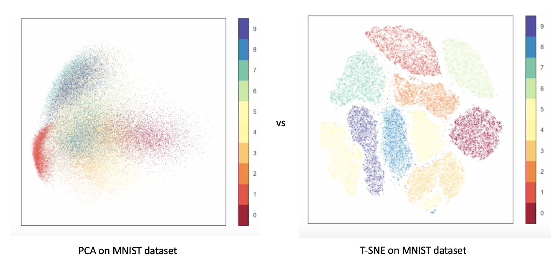 Comparison of t-SNE and UMAP on MNIST dataset. (Image from
 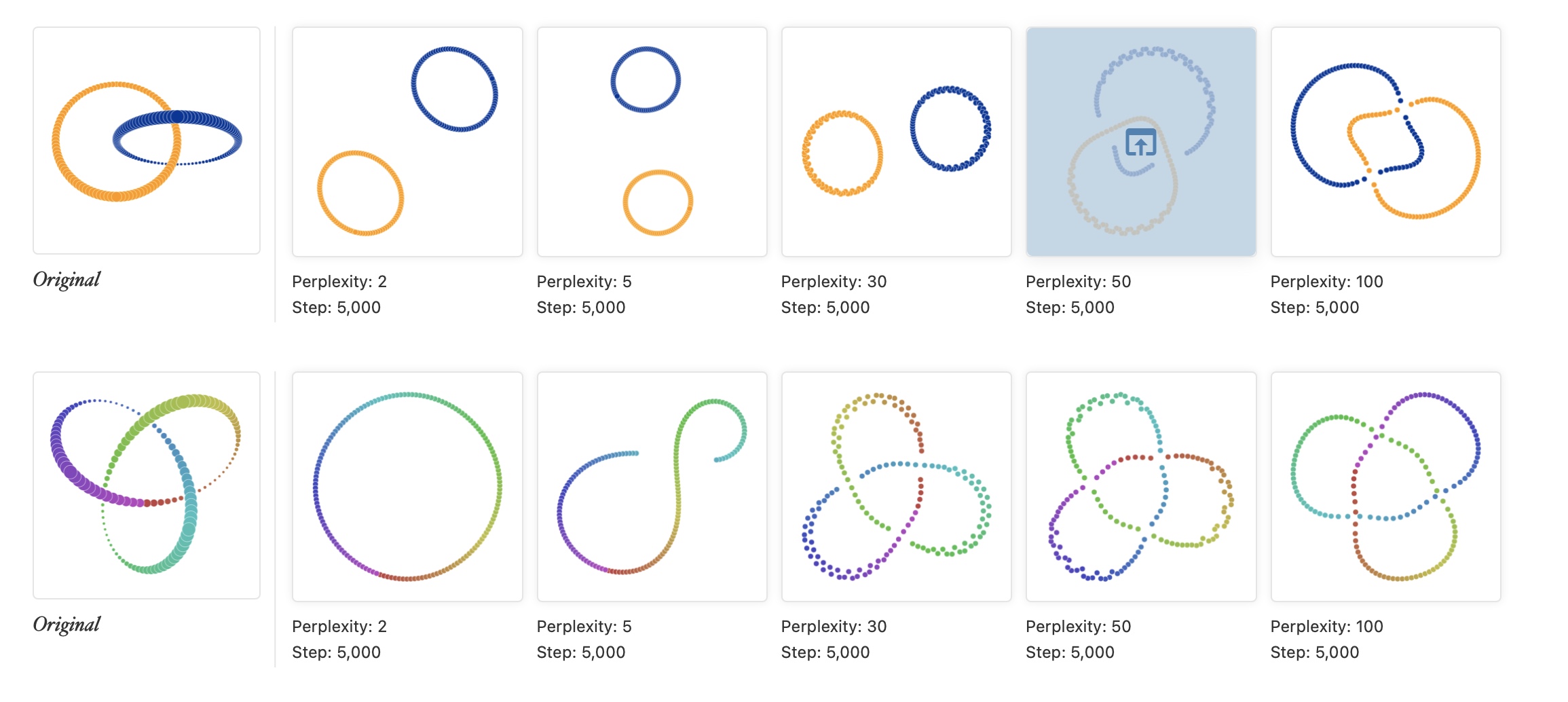 Different patterns are revealed under different t-SNE configurations, as shown by
 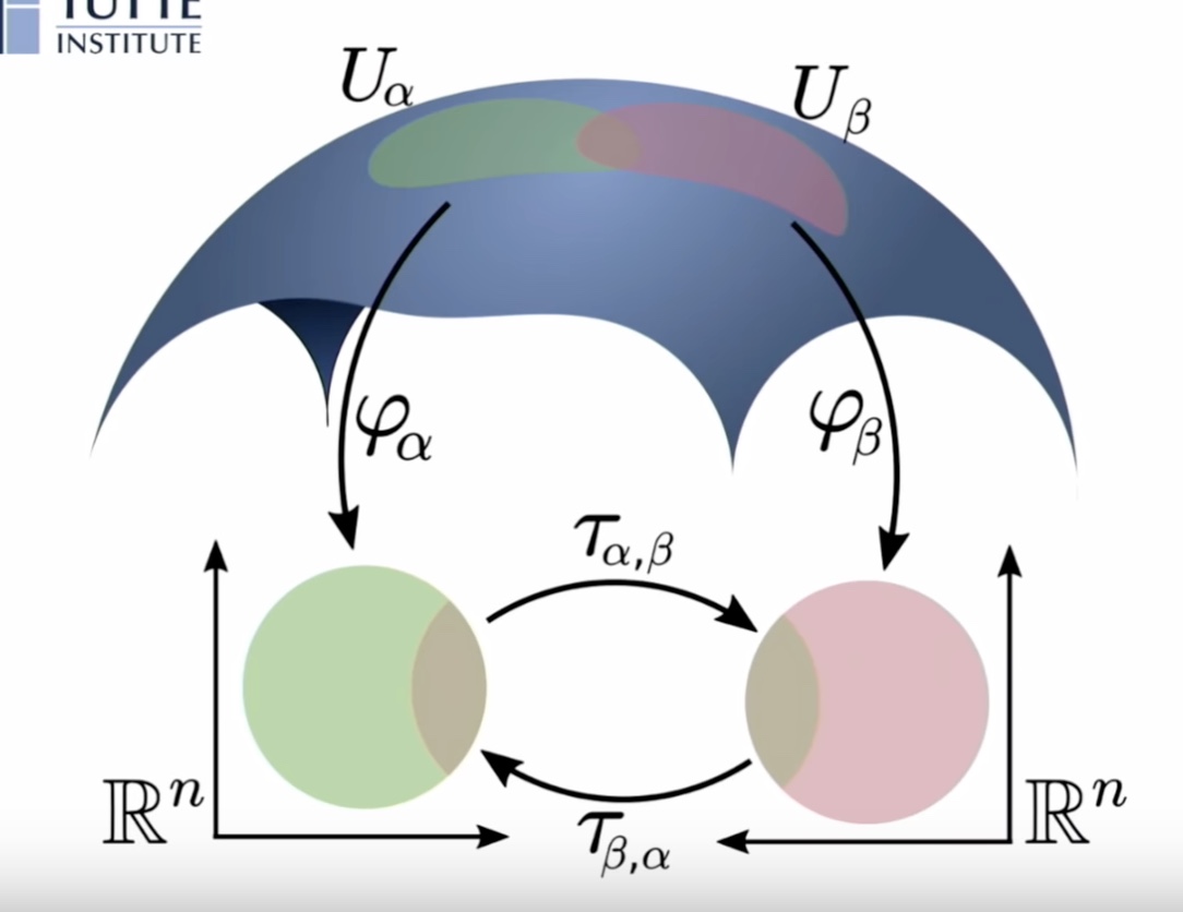 Manifold reprojection used by UMAP, as presented by
 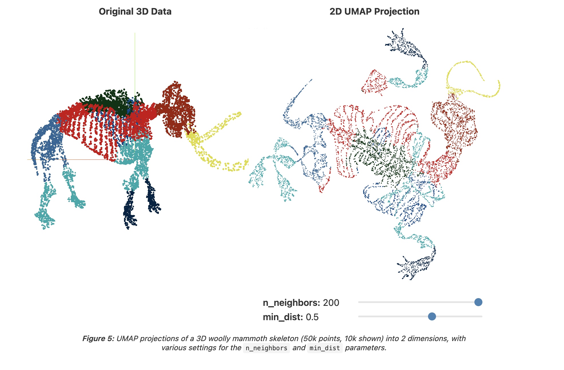 Example of UMAP reprojecting a point-cloud mammoth structure on 2-D space. (Image provided by the author, produced using tool
 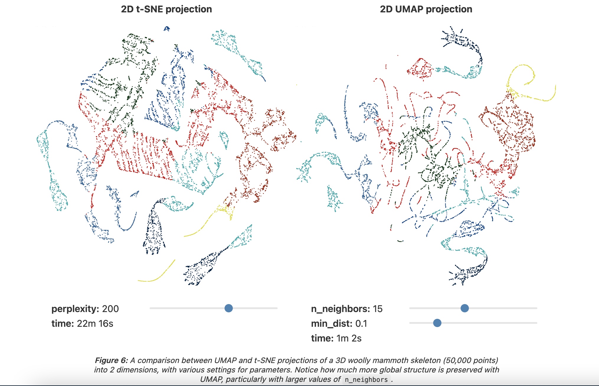 Side by side comparison of t-SNE and UMAP projections of the mammoth data used in the previous figure. (Image provided by the author, produced using tool
 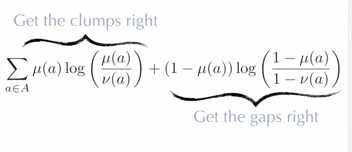 Cots function used in UMAP as discussed in
 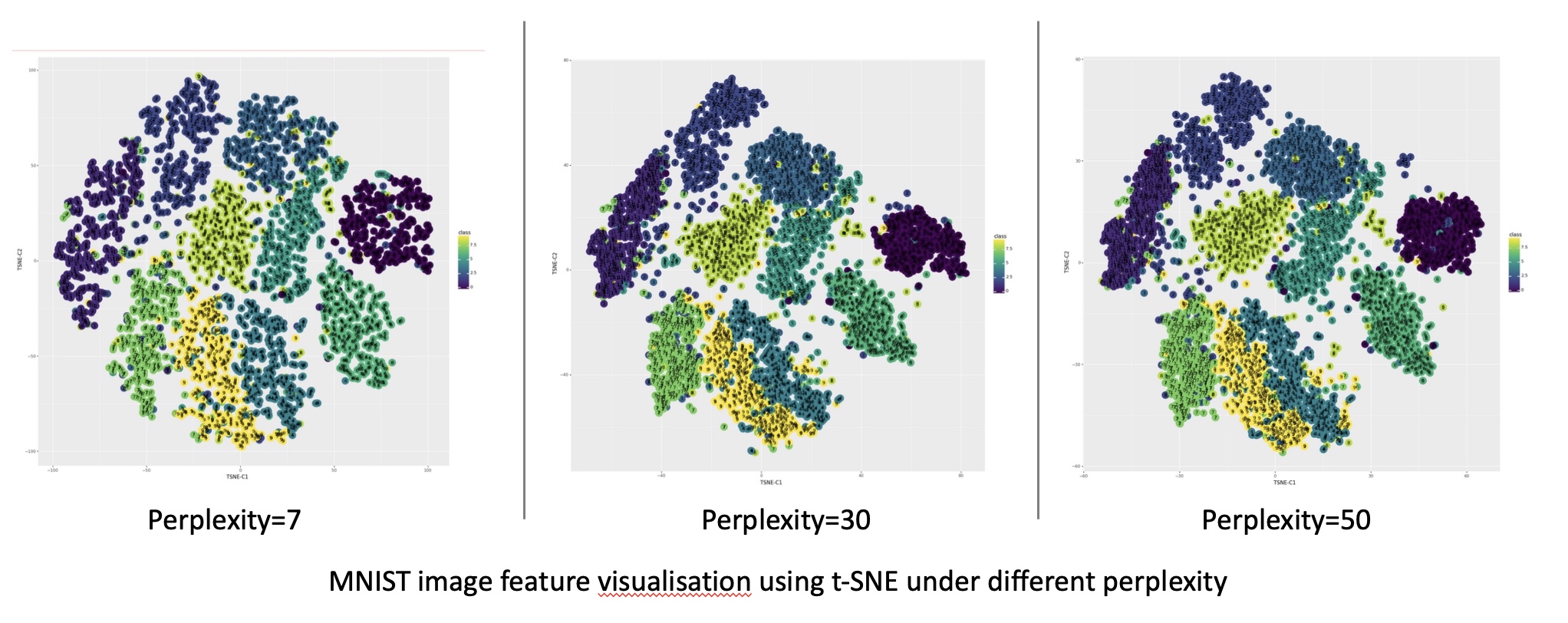 Reprojection of MNIST image features on the 2D embedded space using t-SNE under different perplexity settings. (Image provided by author)
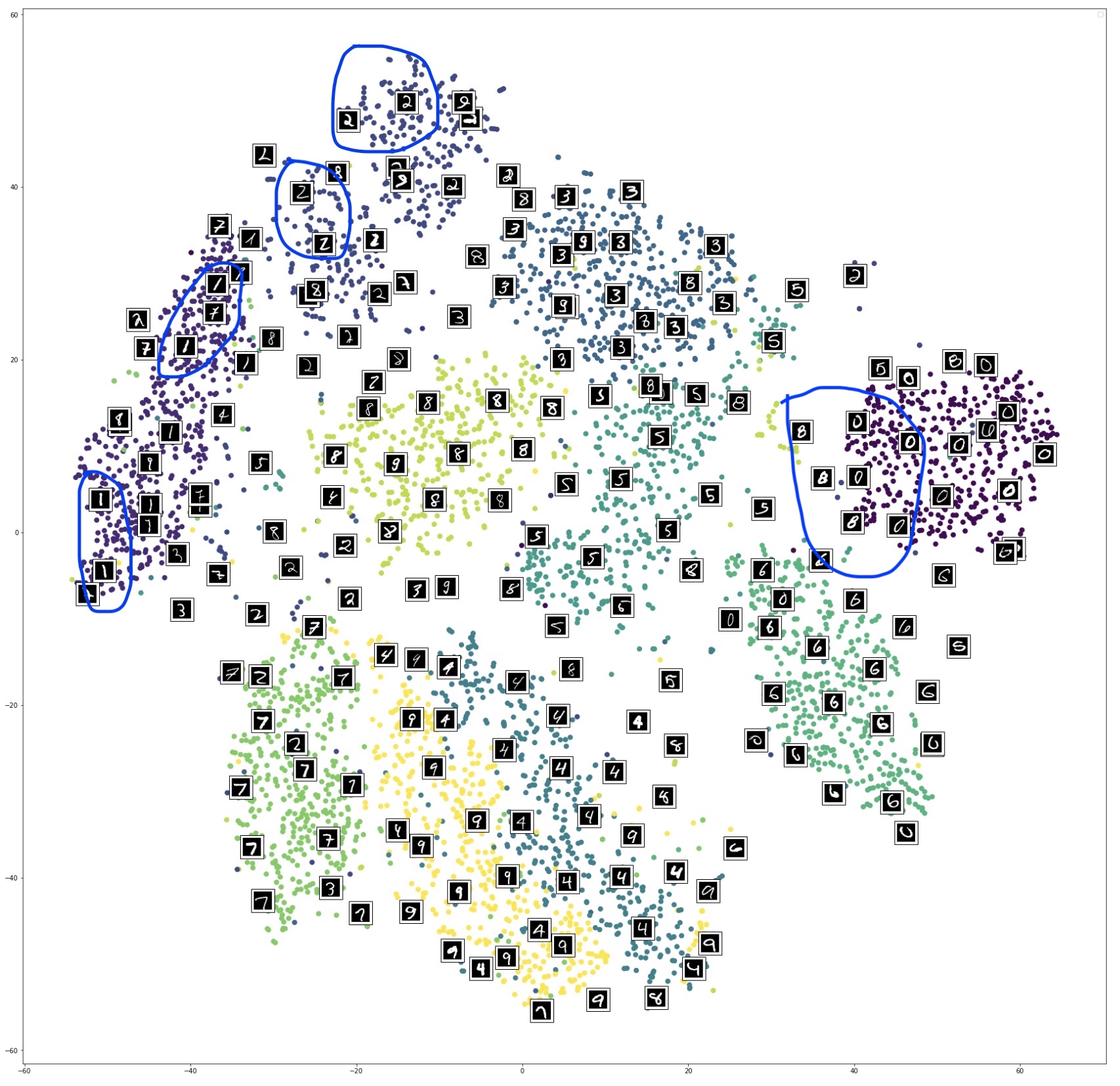 Reprojection of MNIST image features on the 2D embedded space using t-SNE @ perplexity=50 with randomly selected image overlay. (Image provided by author)
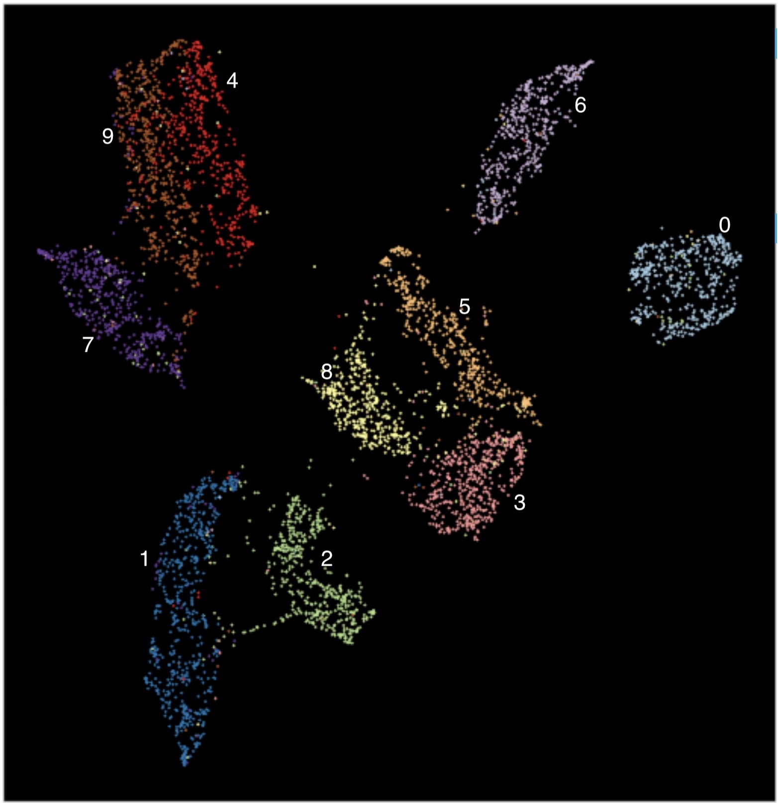 Reprojection of MNIST image features on the 2D embedded space using UMAP. (Image provided by author)
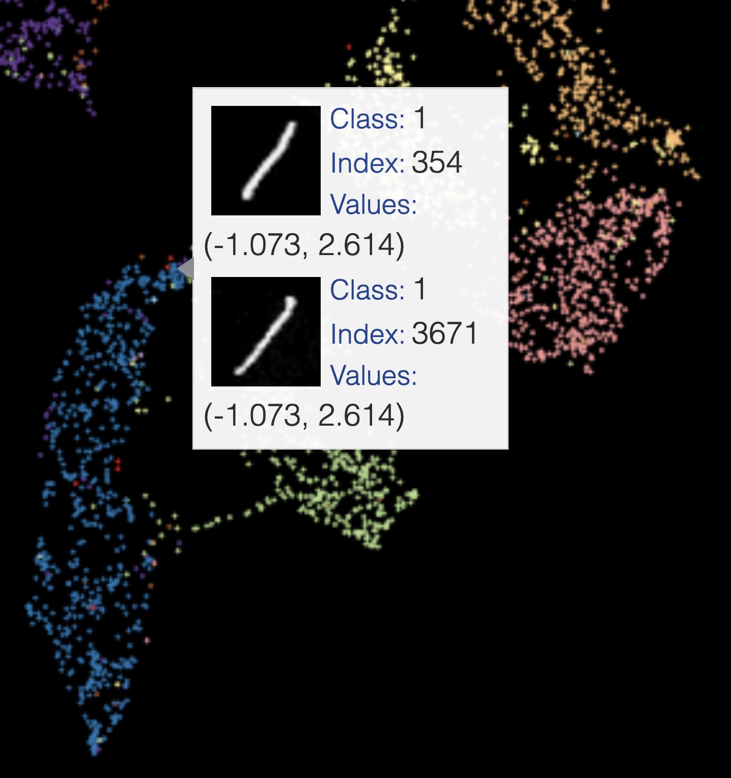 One example of samples that get reprojected to the same coordinates in the embedded space using UMAP. (Image provided by author)
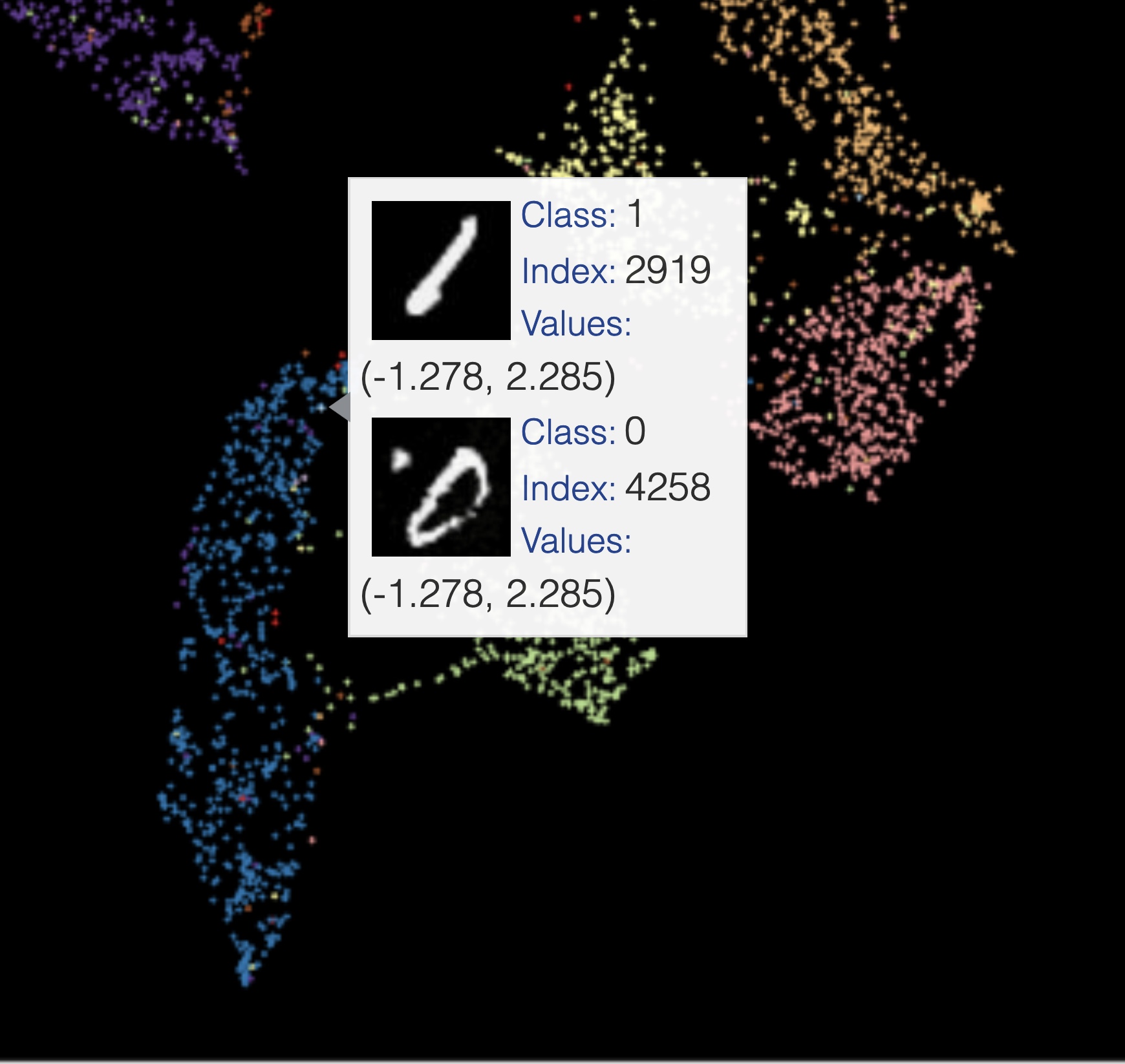 One example of two different digits getting reprojected to the same coordinates in the embedded space using UMAP. (Image provided by author)
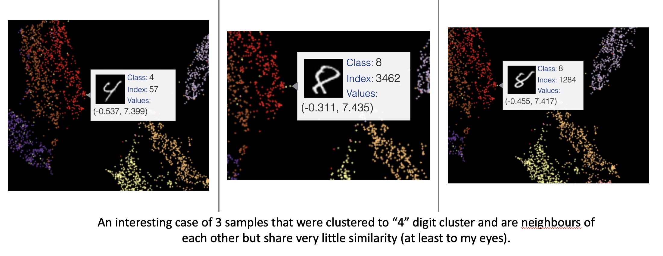 Example of 4 and 8s reprojected to the nearby coordinates in the embedded space using UMAP. (Image provided by author)
 High-level differences between
 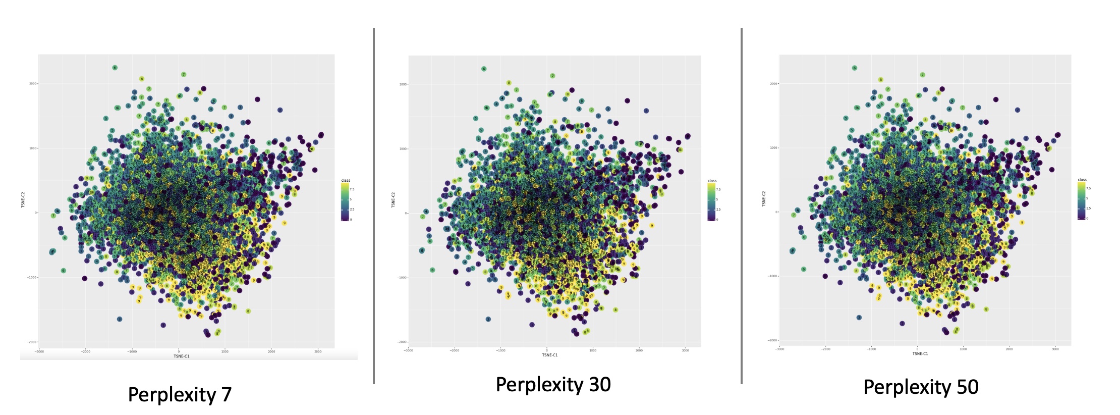 Results of CIFAR image feature visualization using t-SNE under different perplexity settings. (Image provided by author)
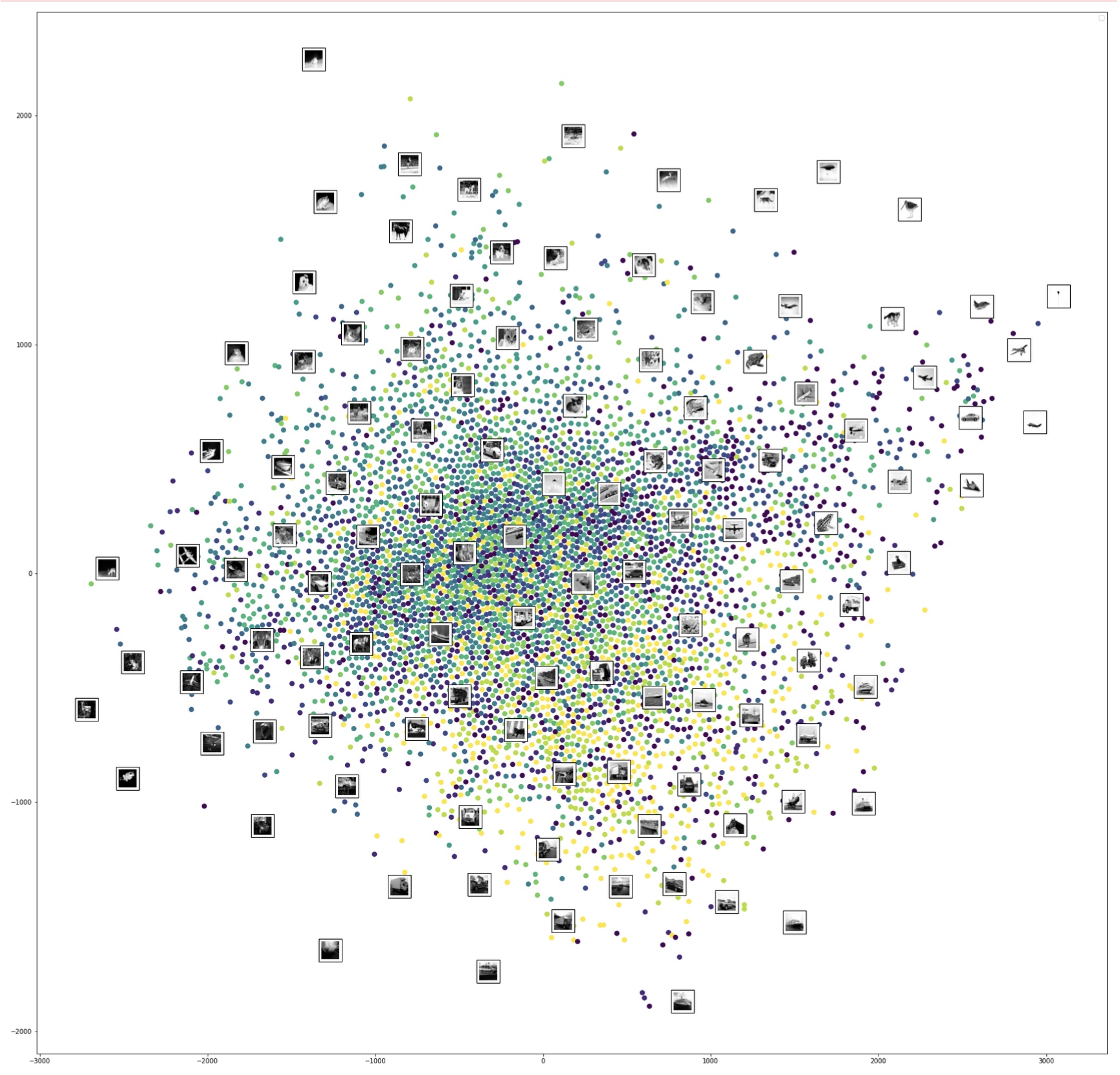 Results of CIFAR image feature visualization using t-SNE. Shows images in an overlay on randomly selected points. (Image provided by author)
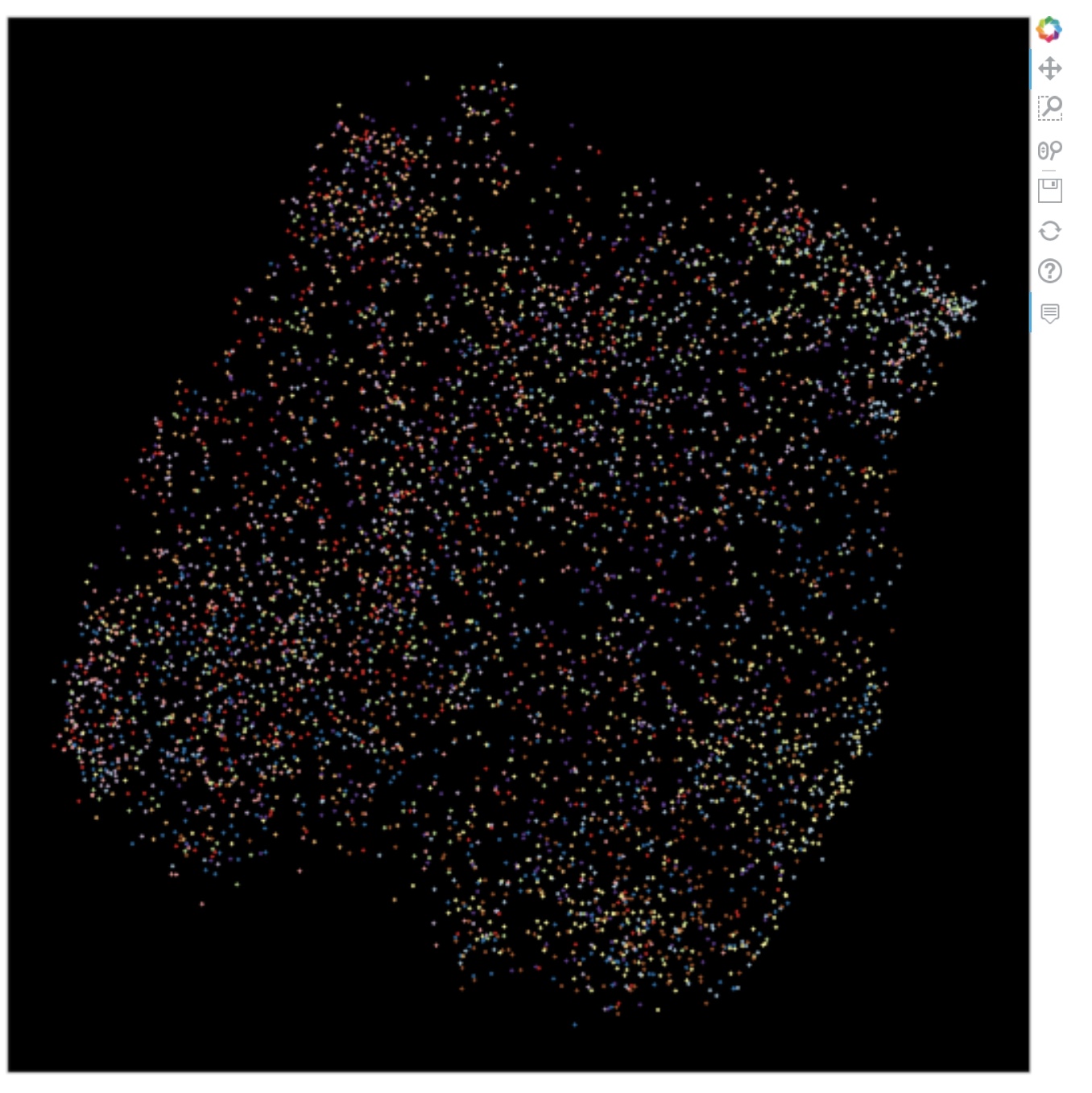 Results of CIFAR image feature visualization using UMAP. (Image provided by author)
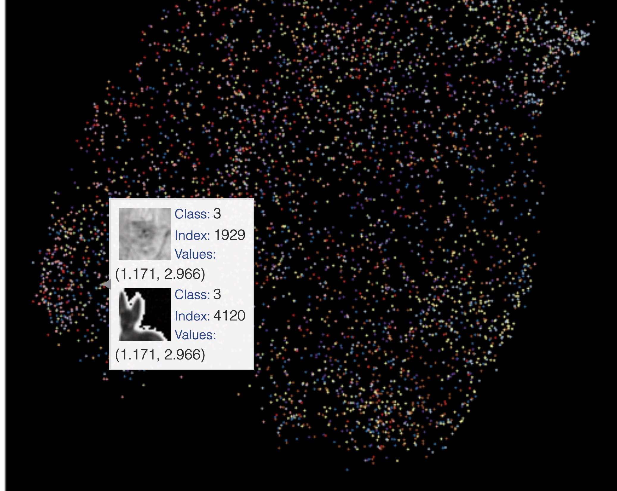 Results of CIFAR image feature visualization using UMAP showing samples of cats that are reprojected into the same located in the embedded space. (Image provided by author)
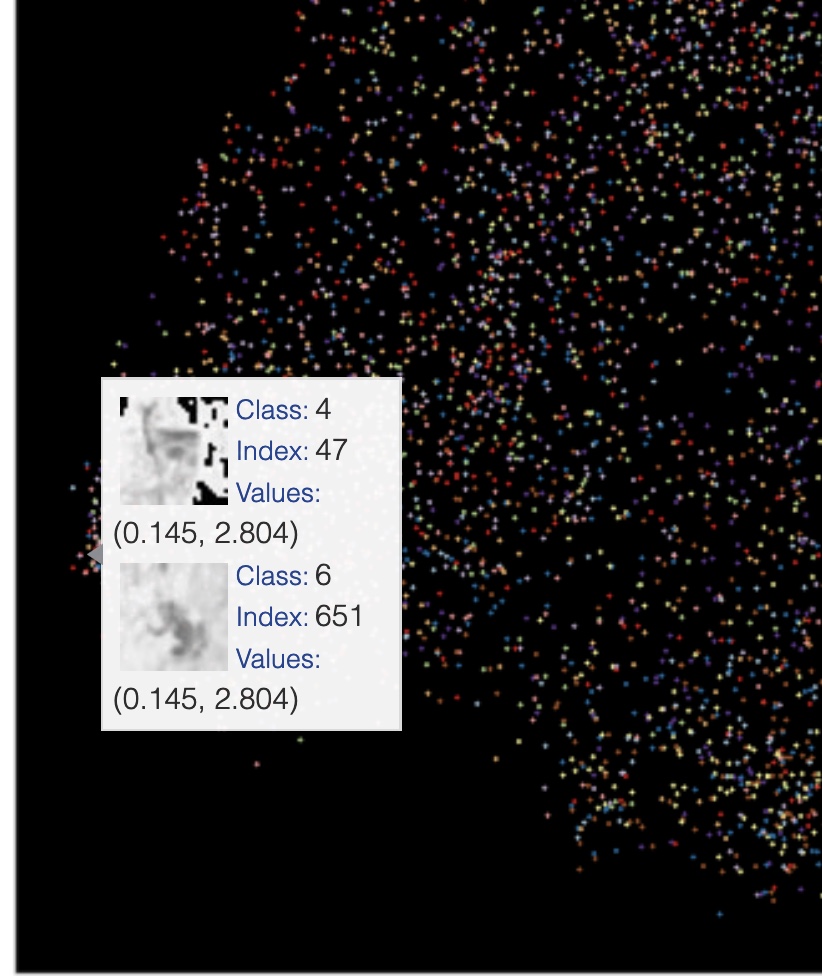 Results of CIFAR image feature visualization using UMAP. Shows images in an overlay on randomly selected points. (Image provided by author)
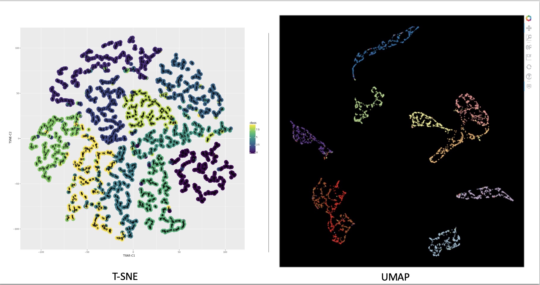 Results of applying autoencoder on MNIST before applying manifold algorithm t-SNE and UMAP. (Image provided by author)
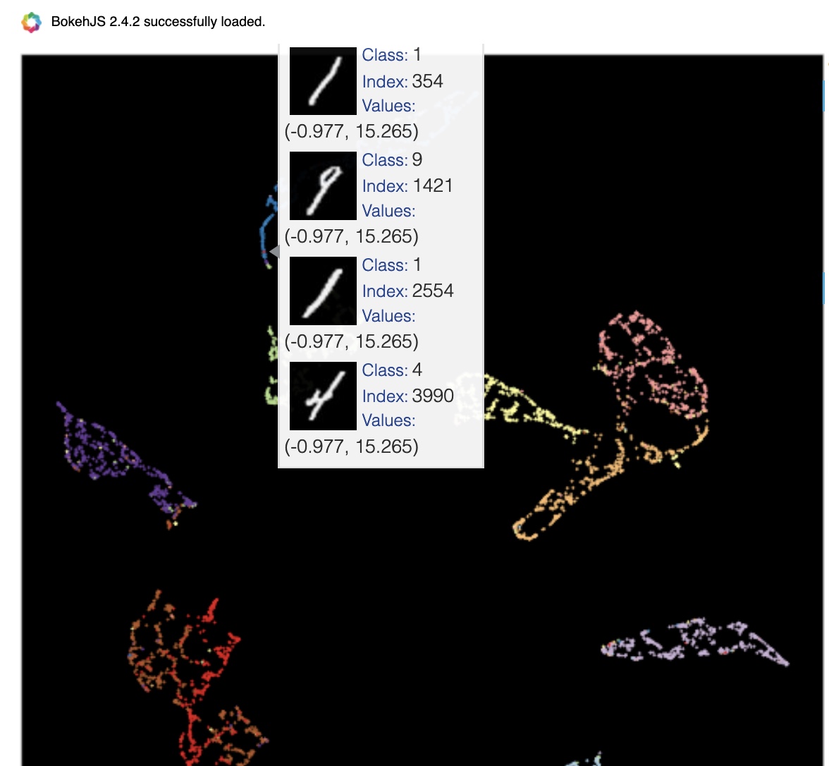 Example of co-located 1s, 4 & 9 in embedded space obtained by applying Paramertic UMAP on MNIST. (Image provided by author)
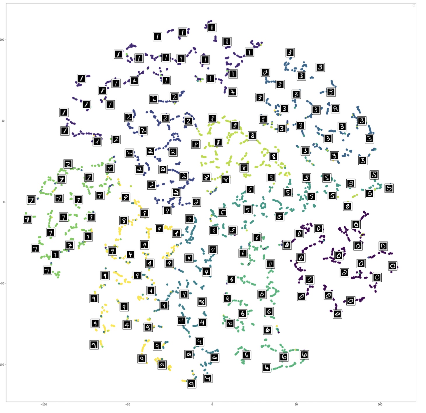 Images overlaid on t-SNE of auto-encoded features derived from MNIST dataset. (Image provided by author)
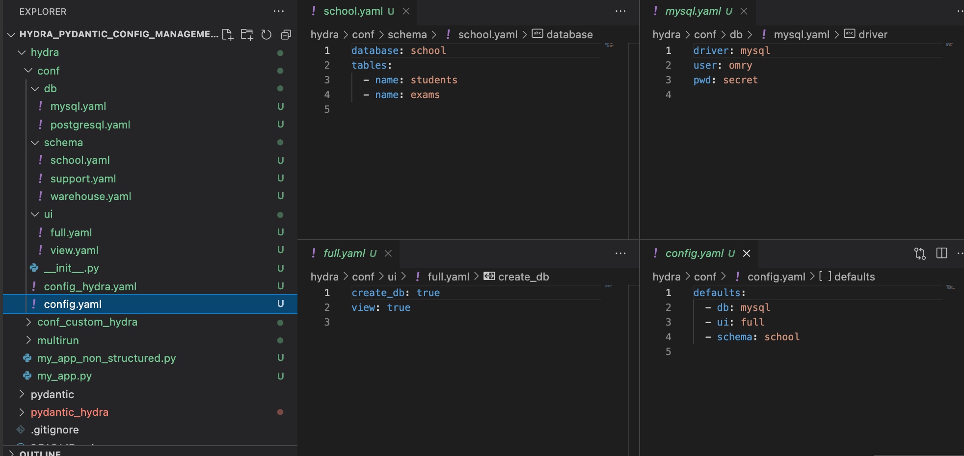 Example hierarchical hydra config.
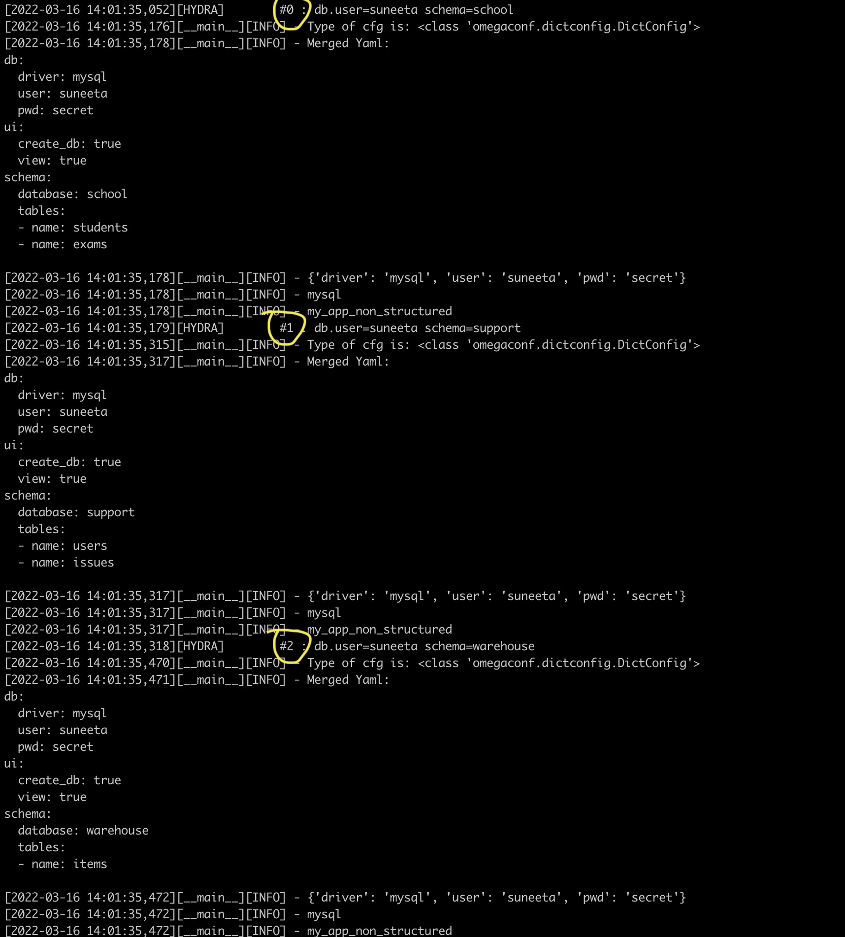 Example Of multi-runs.
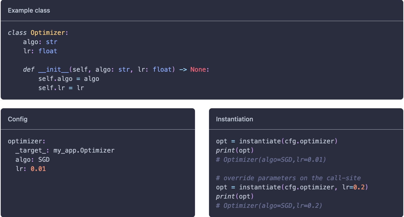 Example Of instantiate objects.
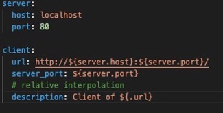 Example Of instantiate objects.
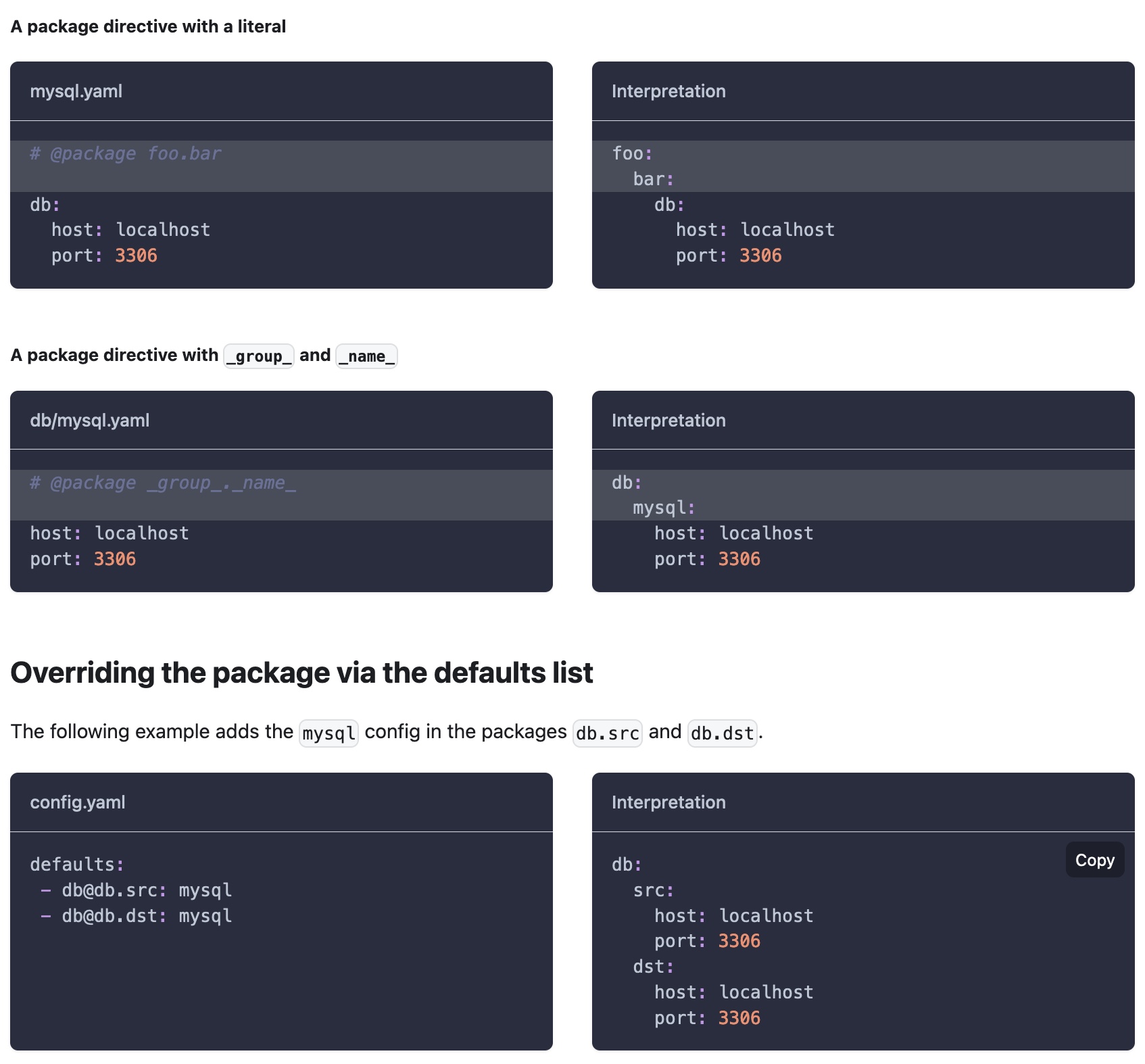 Example Of directives to rewrite config specifications.
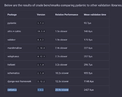 Hydra's benchmarks.

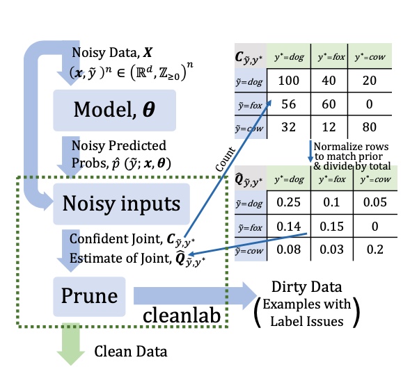
 Borrowed from
 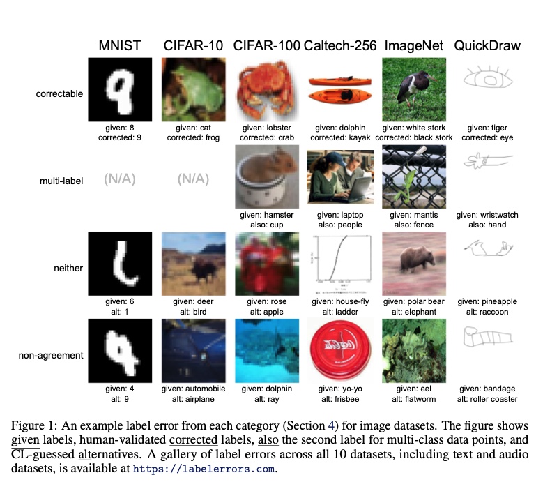 Examples of samples corrected using
 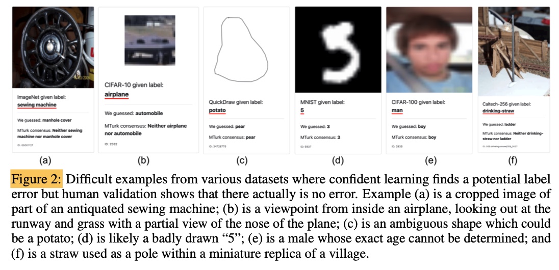 Examples of samples
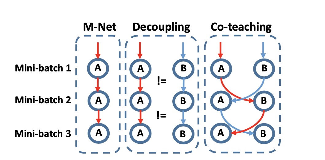
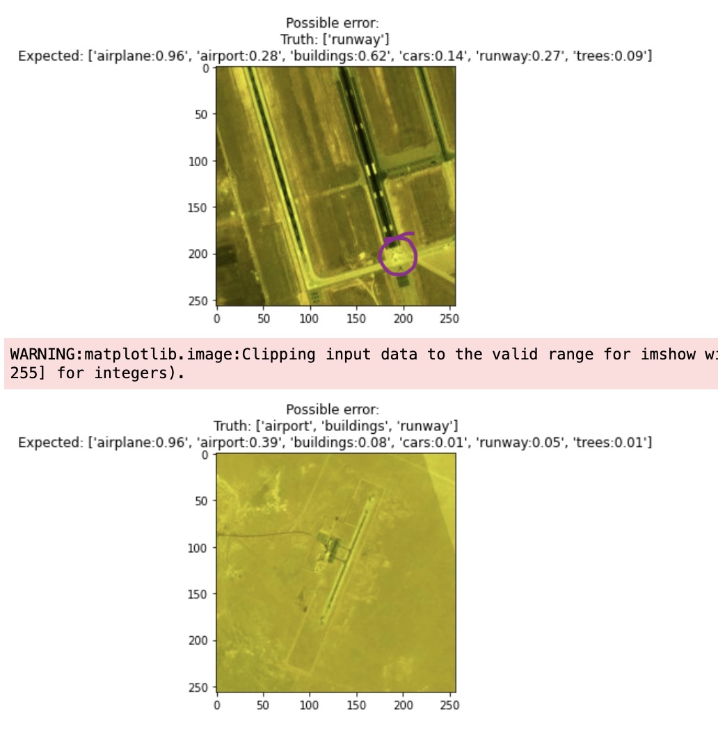
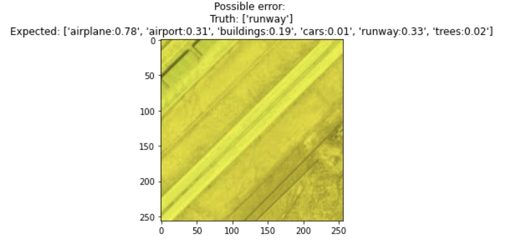
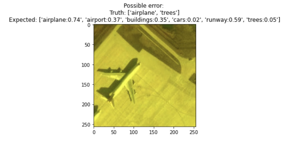
 *Figure 1: Shows relationship between generalization error and dataset size (log scale)
 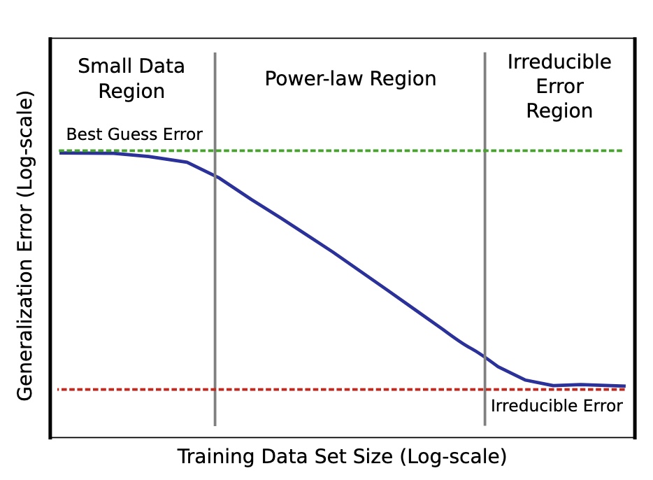 *Figure 2: Power Law curve showing model trained with a small dataset only as good as random guesses to rapidly getting better as dataset size increases to eventually settling into irreducible error region explained by a combination of factors including imperfect data that cause imperfect generalization
 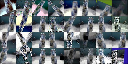 * Example of augmentation
 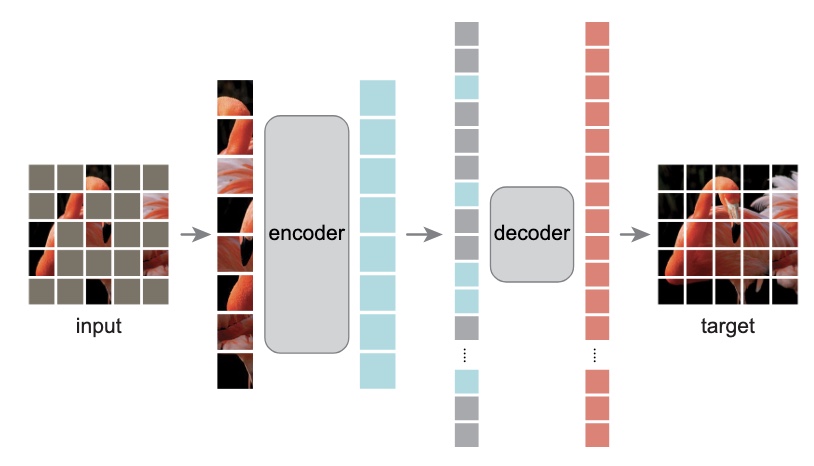 Masked-Autoencoders showing model inferring missing patches
 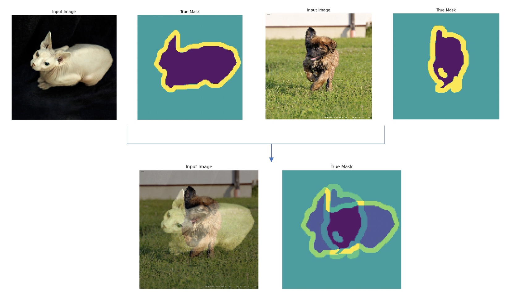 *Figure 4: Sample produced by applying mixup
 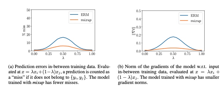 Figure 5: Shows that using mixup
 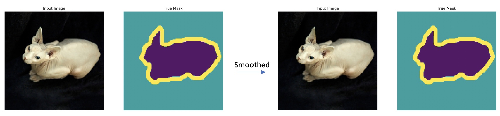 Applying label-smoothing has no noticeable difference
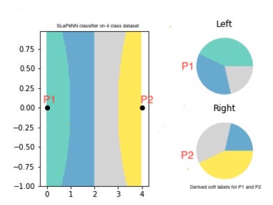 Figure LO-Shot: LO Shot splitting 4 class space into 2 points
 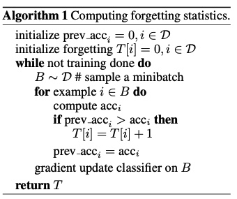 Figure 6: Algorithm to track forgotten samples
 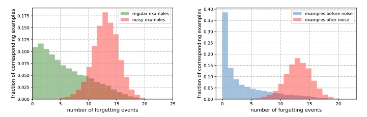 Figure 7: Indicating how increasing fraction of noisy samples led to increased forgetting events
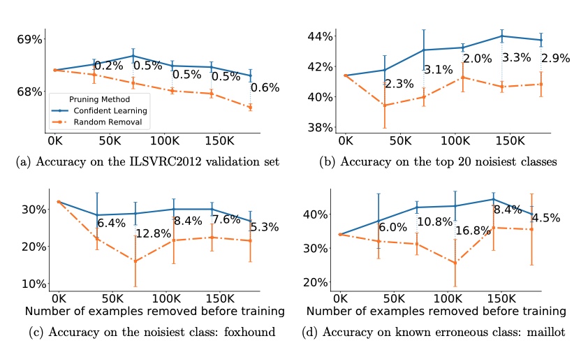
 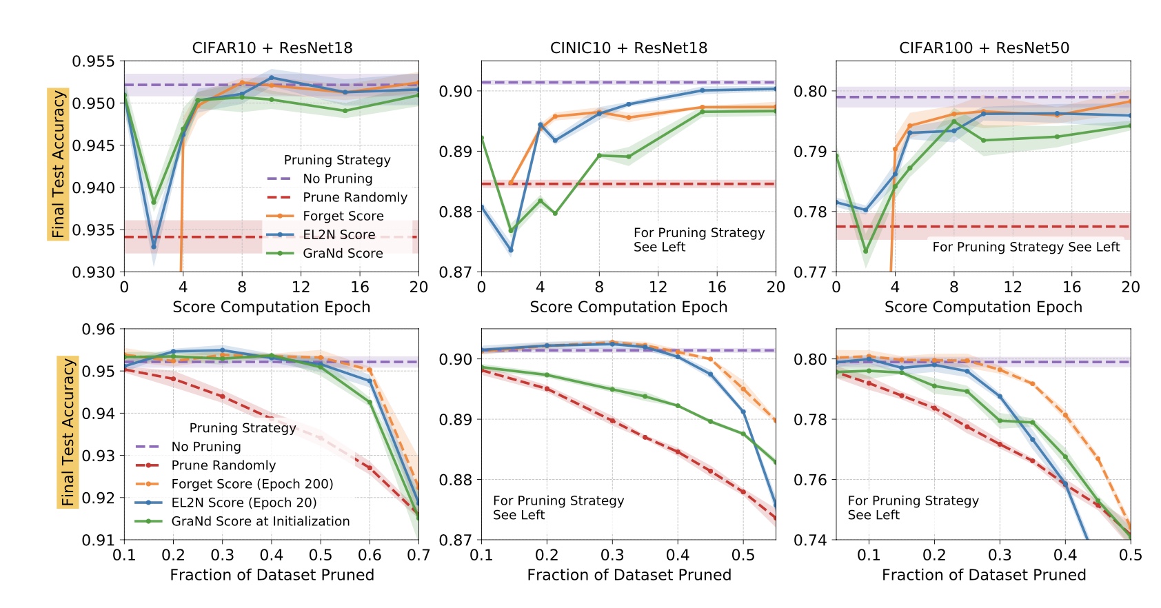 Results of prunning with GradNd and EL2N
 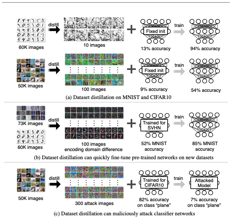 Figure 8: Dataset distillation results from FAIR study
 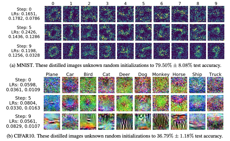 Figure 9: Dataset distillation results from FAIR study
 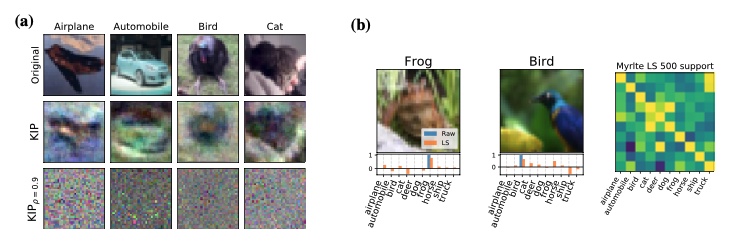 Figure 10: Examples of distilled samples a) with KIP and b) With LS
 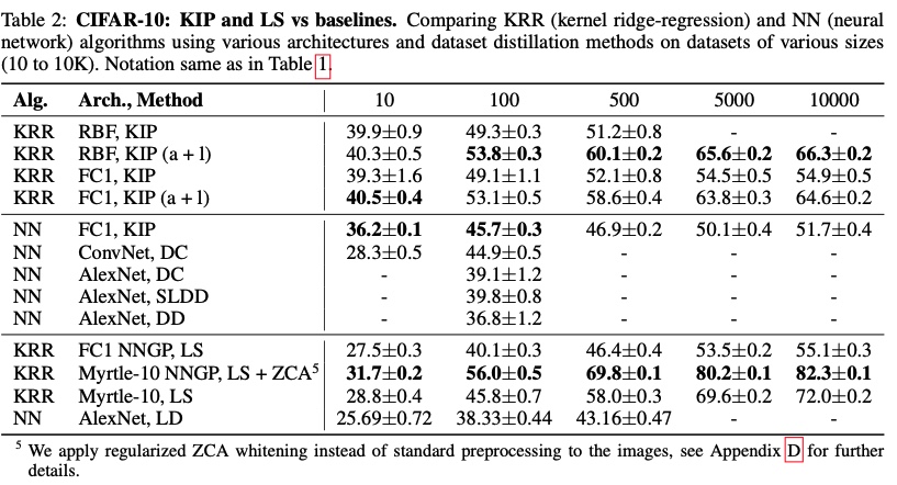 Figure 11: CIFAR10 result from KIP and LS
 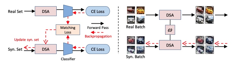 Figure 12: Differentiable Siamese Augmentation
  Figure 13: Infinite width Convolution networks converging to infinity
 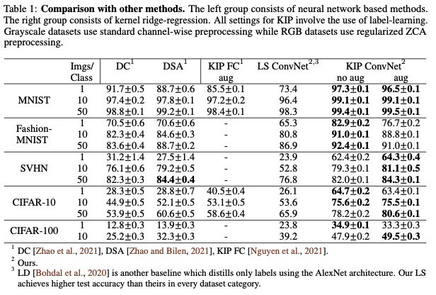 Figure 14: KIP ConvNet results
 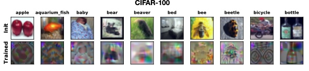 Figure 15: KIP ConvNet example of distilled CIFAR set
 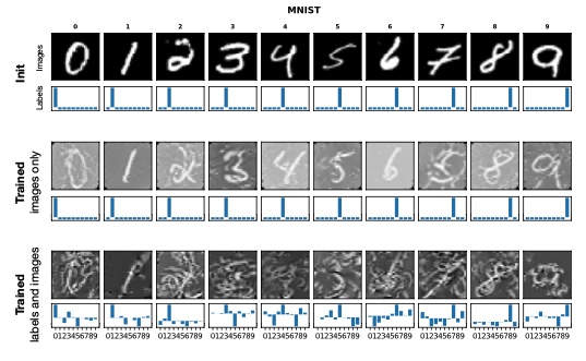 Figure 16: KIP ConvNet example of distilled MNIST set
 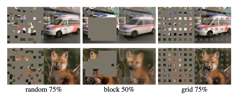 Figure 17: Noisy patches in Masked-AutoEncoder
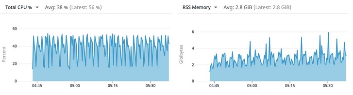 Figure 2: Average resource requirements of the app when run on VMs or bare metal
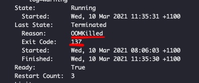 Figure 3: The killer is on the loose! - Whodunit?
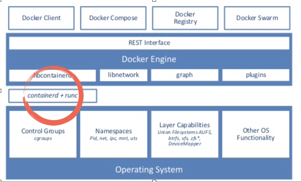 Figure 5: Docker stack! Image credit: internet
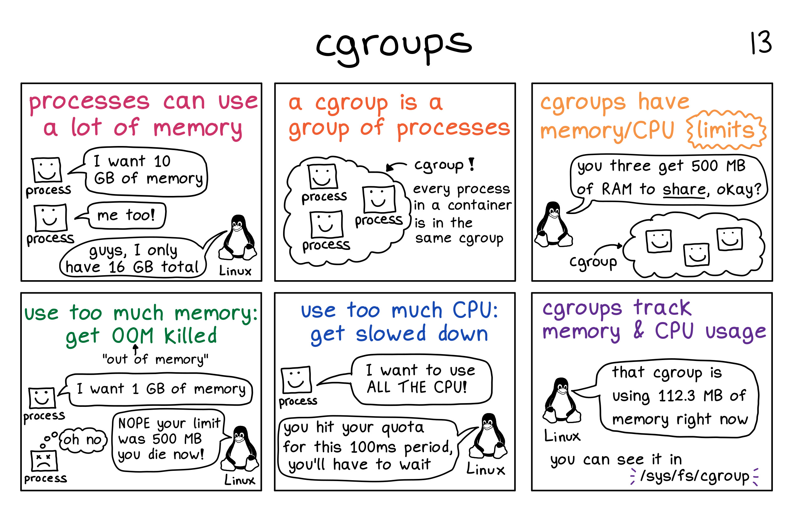 Figure 6: CGroup in picture! Image credit:
 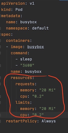 Figure 7: Guaranteed QoS pod example
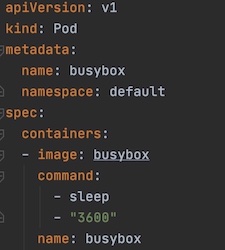 Figure 8: Best-Effort QoS pod example
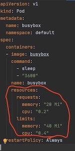 Figure 9: Burstable QoS pod example
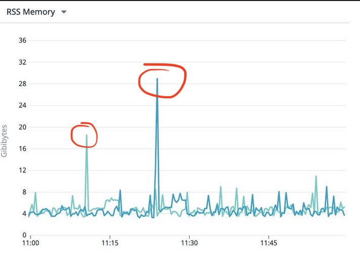 Figure 10: The notorious spike of memory use on pod
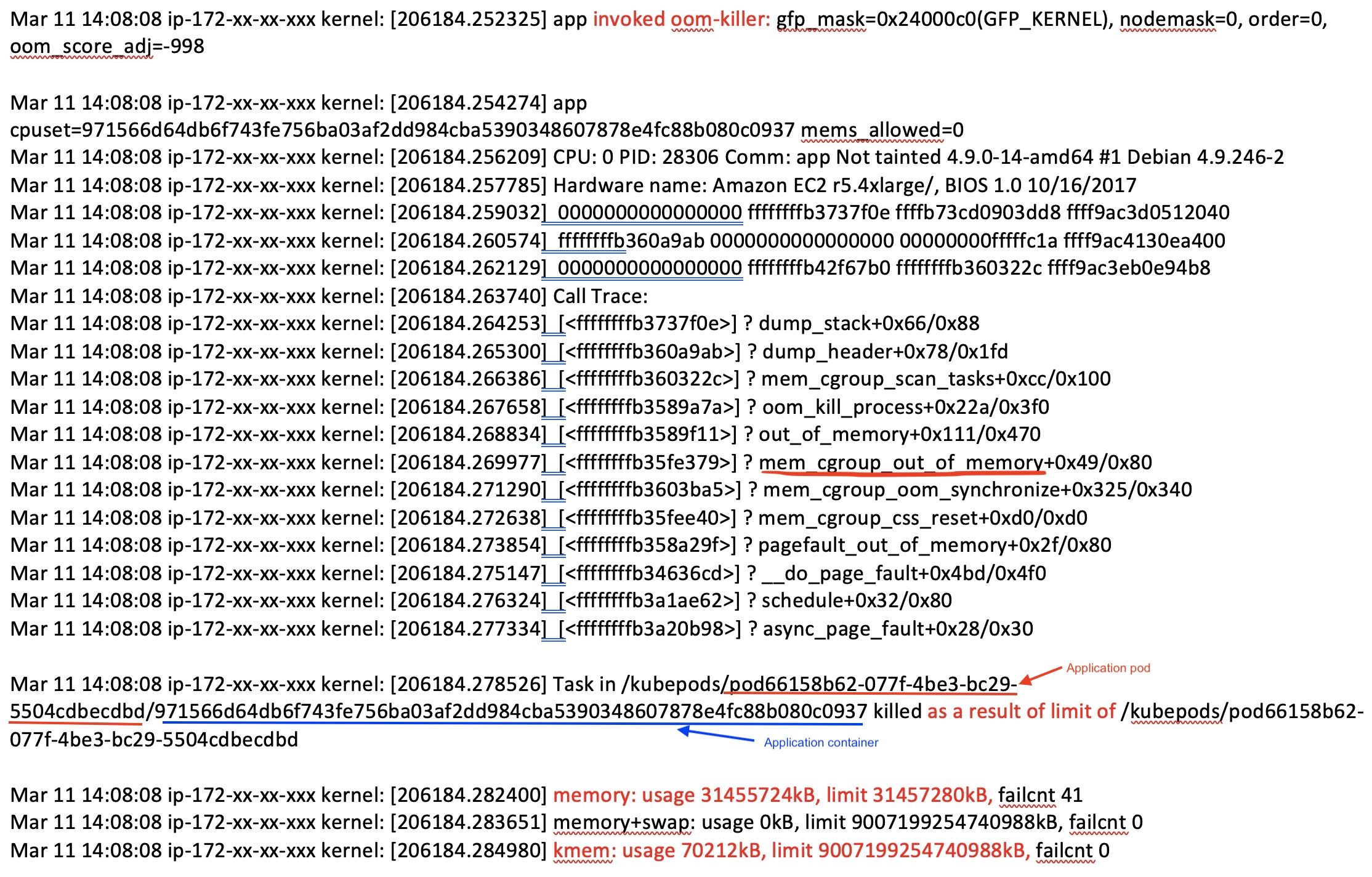 Figure 12: Kernel log part 1
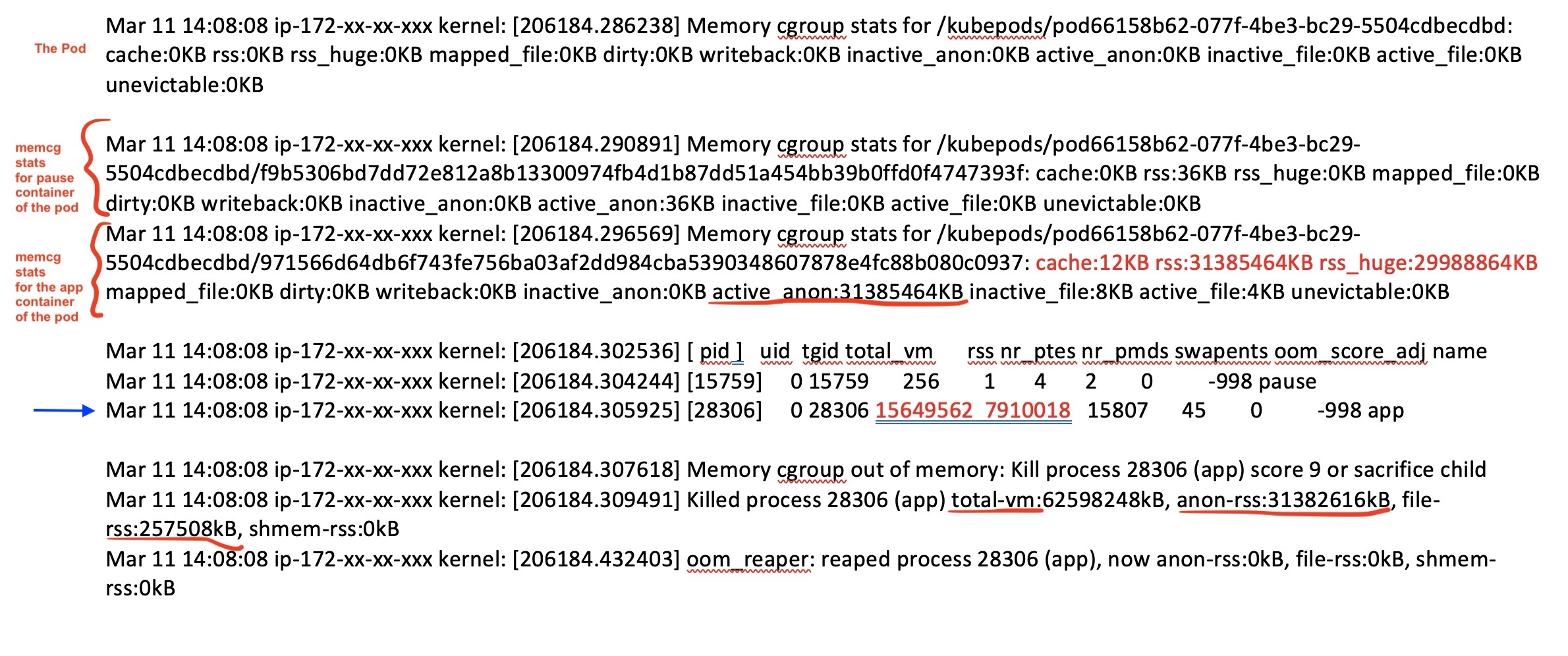 Figure 13: Kernel log part 2

 Figure 14: Getting somewhere! OOMKills sort of under control!